This is a comprehensive research on the supermarket of Bangladesh where we have tried to find out the customers overall view, attitude and their behavior towards the supermarket. Besides, we have tried to implement our knowledge that we have learned so far from this course to find out some inner question answers from the actual customers of supermarket that help us a great deal to come up with some key findings as well as recommendations. This findings and recommendations that we have given after a comprehensive research that will help us and especially the supermarkets of Bangladesh to know that what kind of services they are providing their customers, what should they do to satisfy their customers, and how they will implement these activities to satisfy their customers which will help to boost up their business.
BACKGROUND
This study has been accomplished as an important task of the project work for the Marketing Research course at NorthSouthUniversity under the supervision of our honorable faculty MD. MONIRUZZMAN. Moreover, the objective of this project is to implement of the learning materials in the practical field of work which will prove the understanding of the learning materials. In addition, this work helps us to make a clear understanding about the implementation side of these learning materials in various fields specially using the stat Pac for windows software which will have a great positive impact in our future life.
RESEARCH OBJECTIVES AND GOALS
The main objective of the research is to find out the comprehensive information from the supermarket customers in terms of their attitude, behavior, choice, and different filling including the external and internal feelings when they purchase their grocery items from the supermarkets. In addition, we have some others mottos that we have tried to find out when we collect the data from the supermarket customers which include- the customers demographic profile, there preferences, product range of the supermarket, purchasing frequency, internal and some external facilities that influence a customer to purchase more from supermarket, customer expectation regarding the supermarket service, and the impact of various promotional offers on customers.
MATHOD OF COLLECTING THE DATA
Primary data:
We have collected the primary data from the field survey using the questionnaire from those people who go to the supermarket for their grocery shopping.
Secondary data:
We also collect the secondary data for the assistance of our research work. Besides, for collecting the secondary data we use our book which is provided by our faculty.
RESEARCH METHOLODOGY
The research methodology based on some steps these are as:
Identify the population:
We first identify our population for conducting the research on supermarket of Bangladesh from the vast number of population at Dhaka city.
Determine the sample size:
Then we determine the total sample size 35 among the total population for accomplishing our research. Where we set up some sampling criteria which are as follows:
- Our respondent:
- People who regularly go to the supermarket for their grocery shopping.
- People who have the sufficient financial capability to go to the supermarkets.
- We exclude the people who are under aged and belonging to the minor group.
- Condition of sample
- Sample source: we collect the data for our research from the top five supermarkets that are situated in Dhaka.
OUR MAIN ASSUMPTION OF RESEARCH
Our main assumptions are based on some crucial steps these are as follows:
Customers: Here, our target customers are those people who go to the supermarket in a regular basis for their accomplishment of their grocery shopping.
Targeted supermarkets: Our targeted supermarkets are Agora, PQS, Nandan, Mina Bazaar and Almas.
Chorological steps of the research work
LIMITITIONS OF THE RESEARCH:
- Since this is the research which largely depends on the field survey as a result we have to depend on the survey result. For this reason, in some cases we get the poor result which makes our survey difficult.
- In some cases we don’t get the proper help from the interviews which limit our research capacity.
- In some cases where we had to go to the supermarket and that time we don’t get the proper assistance from the authority which constrain our research capacity.
CORRELATIONS
Stat Pac for windows
Variable in the analysis- Descriptive statistics for analysis:
| Variable | Mean | Std. Deviation | N |
| Household Income | 4.29 | .893 | 35 |
| Top up Expenditure | 3.69 | 1.105 | 35 |
Pearson’s Product-Moment Correlation Matrix
| V3 | ||
| V11 | r | .160 |
| N | 35 | |
| SE | 0.158 | |
| t | 1.222 | |
| p | .135 |
There is a positive correlation between household income (v3) and top up expenditure (V11) and that is .160.
Comment:
It means if people income increase then there top up expenditures will also increase with there income as it is considered to be the daily needed commodity of life.
Variable in the analysis- Descriptive statistics for analysis:
| Variable | Mean | Std. Deviation | N |
| Average Weekly Expenditure ON Both S.M and shops. | 6.83 | 1.043 | 35 |
| Average Weekly Expenditure On S.M | 4.83 | 1.562 | 35 |
Pearson’s Product-Moment Correlation Matrix
| V5 | ||
| V6 | r | .812 |
| N | 35 | |
| SE | 0.084 | |
| t | 5.728 | |
| p | .000 |
There is a positive correlation between average weekly expenditure on both supermarkets and shops (v5) and average weekly expenditure on supermarket product (V6) and that is .812.
Comment:
It means people spend for their regular commodities and grocery products proportionally in both supermarkets and shops.
Variable in the analysis- Descriptive statistics for analysis:
Mean | Std. Deviation | N | |
| Age | 4.37 | 1.330 | 35 |
| Frequency Of Grocery purchasing | 2.29 | .710 | 35 |
Pearson’s Product-Moment Correlation Matrix
| V2 | ||
| V7 | r | -.427 |
| N | 35 | |
| SE | 0.159 | |
| t | 0.224 | |
| p | .873 |
There is a negative correlation between age (v2) and frequency of grocery purchasing (V7) and that is .812.
Comment:
It means there is week relationship between age and frequency of grocery purchasing because any age people can purchase their grocery when it is nodded.
Variable in the analysis- Descriptive statistics for analysis:
Mean | Std. Deviation | N | |
| Travel Time | 2.89 | .832 | 35 |
| Frequency Of Grocery grocery shopping. | 2.29 | .710 | 35 |
Pearson’s Product-Moment Correlation Matrix
| V14 | ||
| V7 | r | .269 |
| N | 35 | |
| SE | 0.137 | |
| t | 2.184 | |
| p | .026 |
There is a positive correlation between travel time (v14) and frequency of grocery purchasing (V7) and that is .269.
Comment:
It means if travel time for the grocery shopping is high then people normally try to less visit in the supermarket for their grocery shopping.
Variable in the analysis- Descriptive statistics for analysis:
Mean | Std. Deviation | N | |
| Gender | 1.57 | .502 | 35 |
| Average Weekly ExpON Both | 6.83 | 1.043 | 35 |
Pearson’s Product-Moment Correlation Matrix
| V1 | ||
| V5 | r | -.481 |
| N | 35 | |
| SE | 0.152 | |
| t | 1.258 | |
| p | .217 |
There is a negative correlation between gender (v1) and average weekly expenditure on both supermarkets and shops (V5) and that is -.481.
Comment:
It means there is week relationship between gender and the average weekly expenditure on both supermarkets and shops because average weekly expenditure for grocery doesn’t depend on the gender.
Variable in the analysis- Descriptive statistics for analysis:
Mean | Std. Deviation | N | |
| Supermarket Most Frequently visit | 2.63 | 1.165 | 35 |
| Top up Sup | 2.77 | 1.165 | 35 |
Pearson’s Product-Moment Correlation Matrix
| V8 | ||
| V10 | r | .867 |
| N | 35 | |
| SE | 0.112 | |
| t | 3.812 | |
| p | .000 |
There is a positive correlation between supermarket most frequently visit (v8) and top up sup (V10) and that is .867.
Comment:
We have seen many people from our survey that they use supermarkets for their grocery shopping as well as their top up shopping as a result there is a positive relationship between the supermarkets most frequently visit and top up supermarket.
Variable in the analysis- Descriptive statistics for analysis:
Mean | Std. Deviation | N | |
| House hold Income | 4.29 | .893 | 35 |
| Promotional Offer | 2.40 | 1.063 | 35 |
Pearson’s Product-Moment Correlation Matrix
| V3 | ||
| V19 | r | .478 |
| N | 35 | |
| SE | 0.154 | |
| t | 0.621 | |
| p | .537 |
There is a positive correlation between house hold Income (v3) and promotional offer (V19) and that is .478.
Comment:
Some customers like the promotional offer as there income level is not so high as a result there is a strong relationship between the promotional offers and the income level.
Variable in the analysis- Descriptive statistics for analysis:
Mean | Std. Deviation | N | |
| Travel Distance | 1.49 | .612 | 35 |
| Alt Search Time | 6.37 | .877 | 35 |
Pearson’s Product-Moment Correlation Matrix
| V13 | ||
| V15 | r | .038 |
| N | 35 | |
| SE | 0.134 | |
| t | 2.871 | |
| p | .008 |
There is a positive correlation between travel distance (v13) and alternative search time (V15) and that is .038.
Comment:
There is a strong relationship between the travel distance and the alternative search time because customers don’t show too much interest to find out an alternative supermarket if it takes too much time to visit.
Variables in the Analysis – Descriptive Statistics for analysis
Mean | Std. Deviation | N | |
| Promotional Offer | 2.40 | 1.063 | 35 |
| Supermarkets Own Product | 2.40 | .736 | 35 |
Pearson’s Product-Moment Correlation Matrix
| V19 | ||
| V20 | r | .241 |
| N | 26 | |
| SE | 0.173 | |
| t | 1.809 | |
| p | .083 |
There is a positive relationship between promotional offer (V19) and the supermarket own product (V20) that is .241.
Comment:
It means there is a strong relationship between the promotional offer and the supermarket own product because if supermarket do more promotional offers then their own product will be more popular to the customers.
Variables in the Analysis – Descriptive Statistics for analysis
Mean | Std. Deviation | N | |
| Household Income | 4.29 | .893 | 35 |
| Average Weekly ExpON Both | 6.83 | 1.043 | 35 |
Pearson’s Product-Moment Correlation Matrix
| V3 | ||
| V5 | r | .780 |
| N | 35 | |
| SE | 0.165 | |
| t | 0.960 | |
| p | .345 |
There is a positive relationship between household income (V3) and the average weekly expenditure on both (V5) that is .780.
Comment
It means there is a strong positive relationship between the household income and the average weekly expenditure on both supermarket and shops because if consumer’s income increases then it is very much natural that they will increase their purchase from both supermarkets and shops.
Variables in the Analysis – Descriptive Statistics for analysis
Mean | Std. Deviation | N | |
| Household Income | 4.29 | .893 | 35 |
| Average Weekly Exp On Supermarkets | 4.83 | 1.562 | 35 |
Pearson’s Product-Moment Correlation Matrix
| V3 | ||
| V6 | r | .584 |
| N | 35 | |
| SE | 0.169 | |
| t | 0.233 | |
| p | .817 |
There is a positive relationship between household income (V3) and the average weekly expenditure on supermarket (V6) that is .584.
Comment:
There is strong positive relationship between the household income and the average weekly expenditure on supermarket because if customers’ incomes increase then they will spend more in supermarket for their grocery shopping.
Variables in the Analysis – Descriptive Statistics for analysis
Mean | N | ||
| Frequency Of Grocery shopping | 2.29 | .710 | 35 |
| Top up Exp | 3.69 | 1.105 | 35 |
| V4 | ||
| V9 | r | -.073 |
| N | 35 | |
| SE | 0.163 | |
| t | 1.072 | |
| p | .287 |
There is a negative relationship between frequency of grocery shopping (V4) and top up expenditure in supermarket (V9) that is -.o73.
Comment:
There is a strong negative relationship between these two because frequency of grocery shopping doesn’t go with the top up expenditure.
Variables in the Analysis – Descriptive Statistics for analysis
Mean | Std. Deviation | N | |
| Household Income | 4.29 | .893 | 35 |
| Shopping Category | 2.11 | 1.409 | 35 |
Pearson’s Product-Moment Correlation Matrix
| V7 | ||
| V11 | r | .015 |
| N | 35 | |
| SE | 0.168 | |
| t | 0.065 | |
| p | .947 |
There is a positive relationship between household income (V7) and shopping category in supermarket (V11) that is .015.
Comment:
It means customers choice for the house hold category products largely depend on the customers income.
Variables in the Analysis – Descriptive Statistics for analysis
Mean | Std. Deviation | N | |
| Gender | 1.57 | .502 | 35 |
| Promotional Offer | 2.40 | 1.063 | 35 |
Pearson’s Product-Moment Correlation Matrix
| V1 | ||
| V19 | r | -.110 |
| N | 35 | |
| SE | 0.168 | |
| t | 0.659 | |
| p | .515 |
There is a negative relationship between gender (V1) and promotional offer of supermarket (V19) that is -.o110.
Comment:
Promotional offer don’t have any strong impact on the gender because if it is grocery shopping then it is the necessary goods for both male and female and they have to purchase it for their normal life leading.
CROSSTAB
WHAT IS THE APPROXIMATE TRAVEL DISTANCE OF YOUR SUPER MARKET FROM YOUR HOME? AND- WHICH FORM OF TRANSPORTATION DO YOU NORMALLY USE TO VISIT YOUR SUPERMARKET?
| WHICH FORM OF TRANSPORTATION DO YOU NORMALLY USE TO GO THE SUPERMARKET? | ||||||
| Number Row % Col % Total % | CAR | ON FOOT | PUBLIC BUS | TAXI | OTHERS | Totals |
| 2 | 1 | 3 | 4 | 4 | ||
| 9 | 9 | 1 | 1 | 5 | ||
| 1=<1MILES | 31.7% | 33.3% | 5.2% | 3.2% | 16.7% | 23 |
| 61.5% | 86.9% | 31.3% | 51.0% | 82.0% | 66.8% | |
| 28.6% | 22.9% | 2.9% | 2.9% | 11.4% | ||
| 3 | 0 | 2 | 0 | 1 | ||
| 2=2MILES | 50.0% | 0.0% | 33.3% | 0.0% | 16.7% | 6 |
| 18.8% | 0.0% | 66.7% | 0.0% | 20.0% | 17.5% | |
| 8.6% | 0.0% | 5.7% | 0.0% | 2.9% | ||
| 0 | 0 | 0 | 1 | 0 | ||
| 3=3MILES | 0.0% | 0.0% | 0.0% | 100.0% | 0.0% | 1 |
| 0.0% | 0.0% | 0.0% | 50.0% | 0.0% | 2.6% | |
| 0.0% | 0.0% | 0.0% | 2.9% | 0.0% | ||
| 2 | 1 | 0 | 0 | 0 | ||
| 4=4-5MILES | 66.7% | 33.3% | 0.0% | 0.0% | 0.0% | 3 |
| 12.5% | 11.1% | 0.0% | 0.0% | 0.0% | 8.9% | |
| 5.7% | 2.9% | 0.0% | 0.0% | 0.0% | ||
| 1 | 0 | 0 | 0 | 0 | ||
| 5=>5MILES | 100.0% | 0.0% | 0.0% | 0.0% | 0.0% | 1 |
| 6.3% | 0.0% | 0.0% | 0.0% | 0.0% | 4.2% | |
| 2.9% | 0.0% | 0.0% | 0.0% | 0.0% | ||
| Totals | 16 | 9 | 3 | 2 | 5 | 35 |
| 45.7% | 25.7% | 8.6% | 5.7% | 14.3% | 100.0% | |
Chi-Square = 25.39 Valid Cases = 35
Caution: 23 cells (93%) E<5 Missing Cases = 0
Probability (DF =16) = 0.045 Response Rate = 100.0%
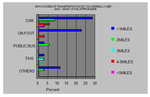
If we describe this curve then we can see the following things these are as follows
- Almost 28% people use the car, 22% use foot, 3% use public bus, 2% use taxi, and 12% use other way as their form of transport to go to the supermarket where there home distance is within one mile.
- Almost 9% people use car, 6% use public bus, 3% people use other way as their form of transport to go to the supermarket where distance is 2 miles.
- Almost 4% people use the taxi to go to the supermarket where distance is 3 miles.
- Almost 6% people use the car to go to the supermarket where distance is 4 miles.
- Almost 3% people use car the others sources to go to the supermarket where distance is more than 5 miles.
HOW OFTEN DO YOU CARRY OUT YOUR MAIN GROCESSARY SHOPPING FROM SUPERMARKET? – AND – WHAT IS THE APPROXIMATE TRAVEL DISTANCE OF YOUR SUPER MARKET FROM YOUR HOME?
| WHAT IS THE APPROXIMATE TRAVEL DISTANCE OF THE SUPER MARKET FROM YOUR HOME? | ||||||
| Number Row % Col % Total % | <1MILES | 2MILES | 3MILES | 4-5MILES | >5MILES | Totals |
| 1 | 2 | 3 | 4 | 5 | ||
| 7 | 3 | 0 | 0 | 0 | ||
| 1=>ONCE A WEEK | 70.0% | 30.0% | 0.0% | 0.0% | 0.0% | 10 |
| 29.2% | 50.0% | 0.0% | 0.0% | 0.0% | 27.5% | |
| 20.0% | 8.6% | 0.0% | 0.0% | 0.0% | ||
| 10 | 2 | 1 | 1 | 0 | ||
| 2=WEEKLY | 71.4% | 14.3% | 7.1% | 7.1% | 0.0% | 14 |
| 41.7% | 33.3% | 100.0% | 33.3% | 0.0% | 39.5% | |
| 28.6% | 5.7% | 2.9% | 2.9% | 0.0% | ||
| 4 | 0 | 0 | 0 | 0 | ||
| 3=FORTNIGHTLY | 100.0% | 0.0% | 0.0% | 0.0% | 0.0% | 4 |
| 16.7% | 0.0% | 0.0% | 0.0% | 0.0% | 11.7% | |
| 11.4% | 0.0% | 0.0% | 0.0% | 0.0% | ||
| 3 | 1 | 0 | 2 | 1 | ||
| 4=MONTHLY | 42.9% | 14.3% | 0.0% | 28.6% | 14.3% | 7 |
| 12.5% | 16.7% | 0.0% | 66.7% | 100.0% | 21.3% | |
| 8.6% | 2.9% | 0.0% | 5.7% | 2.9% | ||
| Totals | 24 | 6 | 1 | 3 | 1 | 35 |
| 68.6% | 17.1% | 2.9% | 8.6% | 2.9% | 100.0% | |
Chi-Square = 12.09 Valid Cases = 35
Caution: 18 cells (89%) E<5 Missing Cases = 0
Probability (DF=12) = 0.368 Response Rate = 100.0%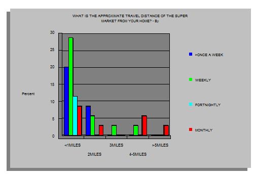
If we describe this curve then we can see the following things these are as follows:
- Almost 66% of the supermarkets customer’s home distance is less than 1 mille whom purchase grocery once a week, weekly, fortnightly, and monthly basis..
- Almost 22% of the supermarkets customer’s home distance is within 2 miles whom purchase grocery once a week, weekly, and monthly basis.
- Almost 4% of the supermarkets customer’s home distance is within 3 miles whom purchase grocery in a weekly basis.
- Almost 10% of the supermarket customers where there home distance is within 4-5 miles and they like to purchase weekly as well as in monthly basis.
- Almost 3% of the supermarket customers where there home distance is more than 5 miles and they like to purchase in monthly basis.
WHAT IS YOUR HOUSEHOLD INCOME? – AND – WHAT IS YOUR REACTION TOWARDS THE SUPAR MARKET PROMOTIONAL TOOLS?
| WHAT IS YOUR REACTION TOWARDS SUPAR MARKET PROMOTIONS? | ||||
| Number Row % Col % Total % | LOOK OUT FOR PROMOTION AND TAKE ADVANTAGE | DO NOT DELIBARATELY SEEK PROMOTION | NEVR NOTICE PROMOTIONS | Totals |
| 1 | 2 | 3 | ||
| 0 | 1 | 0 | ||
| 1=<10000 | 0.0% | 100.0% | 0.0% | 1 |
| 0.0% | 4.5% | 0.0% | 2.9% | |
| 0.0% | 2.9% | 0.0% | ||
| 0 | 1 | 0 | ||
| 2=10000-17… | 0.0% | 100.0% | 0.0% | 1 |
| 0.0% | 4.5% | 0.0% | 2.9% | |
| 0.0% | 2.9% | 0.0% | ||
| 1 | 3 | 0 | ||
| 3=17001-30… | 25.0% | 75.0% | 0.0% | 4 |
| 14.3% | 13.6% | 0.0% | 11.4% | |
| 2.9% | 8.6% | 0.0% | ||
| 2 | 6 | 1 | ||
| 4=31000-50… | 22.2% | 66.7% | 11.1% | 9 |
| 28.6% | 27.3% | 16.7% | 25.7% | |
| 5.7% | 17.1% | 2.9% | ||
| 4 | 11 | 5 | ||
| 5=>50000 | 20.0% | 55.0% | 25.0% | 20 |
| 57.1% | 50.0% | 83.3% | 57.1% | |
| 11.4% | 31.4% | 14.3% | ||
| Totals | 7 | 22 | 6 | 35 |
| 20.0% | 62.9% | 17.1% | 100.0% | |
Chi-Square = 3.36 Valid Cases = 35
Caution: 13 cells (88%) E<5 Missing Cases = 0
Probability (DF=8) = 0.958 Response Rate = 100.0%
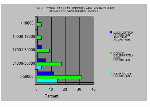
If we describe this curve then we can see the following things these are as follows:
- Almost 64% people do not deliberately seek the promotion of the supermarket.
- Almost 20% people look out for the promotion of supermarket and try to grab the advantage form these kind of advertisement.
- Almost 16% of people never notice the promotional offer of the supermarket and most of them are aged people.
WHT IS YOUR HOUSEHOLD INCOME? – AND – HOW MUCH YOU WANT TO SPEND ON GROCERIES PER WEEK IN BOTH SUPERMARKET AND SHOPS?
| HOW MUCH DO YOU SPEND ON GROCERIES PER WEEK? | |||||||
| Number Row % Col % Total % | 410-500 | 510-750 | 760-1000 | 1010-1250 | >1250 | DON’T KNOW | Totals |
| 4 | 5 | 6 | 7 | 8 | 9 | ||
| 1 | 0 | 0 | 0 | 0 | 0 | ||
| 1=<10000 | 100.0% | 0.0% | 0.0% | 0.0% | 0.0% | 0.0% | 1 |
| 100.0% | 0.0% | 0.0% | 0.0% | 0.0% | 0.0% | 2.9% | |
| 2.9% | 0.0% | 0.0% | 0.0% | 0.0% | 0.0% | ||
| 0 | 1 | 0 | 0 | 0 | 0 | ||
| 2=10000-17… | 0.0% | 100.0% | 0.0% | 0.0% | 0.0% | 0.0% | 1 |
| 0.0% | 25.0% | 0.0% | 0.0% | 0.0% | 0.0% | 2.9% | |
| 0.0% | 2.9% | 0.0% | 0.0% | 0.0% | 0.0% | ||
| 0 | 0 | 0 | 4 | 0 | 0 | ||
| 3=17001-30… | 0.0% | 0.0% | 0.0% | 100.0% | 0.0% | 0.0% | 4 |
| 0.0% | 0.0% | 0.0% | 36.4% | 0.0% | 0.0% | 11.4% | |
| 0.0% | 0.0% | 0.0% | 11.4% | 0.0% | 0.0% | ||
| 0 | 1 | 3 | 1 | 4 | 0 | ||
| 4=31000-50… | 0.0% | 11.1% | 33.3% | 11.1% | 44.4% | 0.0% | 9 |
| 0.0% | 25.0% | 100.0% | 9.1% | 26.7% | 0.0% | 25.7% | |
| 0.0% | 2.9% | 8.6% | 2.9% | 11.4% | 0.0% | ||
| 0 | 2 | 0 | 6 | 11 | 1 | ||
| 5=>50000 | 0.0% | 10.0% | 0.0% | 30.0% | 55.0% | 5.0% | 20 |
| 0.0% | 50.0% | 0.0% | 54.5% | 73.3% | 100.0% | 57.1% | |
| 0.0% | 5.7% | 0.0% | 17.1% | 31.4% | 2.9% | ||
| Totals | 1 | 4 | 3 | 11 | 15 | 1 | 35 |
| 2.9% | 11.4% | 8.6% | 31.4% | 42.9% | 2.9% | 100.0% | |
Chi-Square = 62.57 Valid Cases = 35
Caution: 28 cells (92%) E<5 Missing Cases = 0
Probability (DF=20) = 0.000 Response Rate = 100.0%
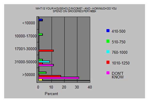
If we describe this curve then we can see the following things these are as follows:
- Almost 32% people income range is more than 50000 taka and they spend more than 1250 taka in a week at both supermarket and shops.
- Almost 14% people income range is in between 31000-50000 taka and they spend more than 1010 taka in a week at both supermarket and shops.
- Almost 12% income range is in between 17001-30000 taka and they spend more than 750 taka in a week at both supermarket and shops.
- Almost 7% people income range is in between 10000-17000 taka and they spend more than 500 taka in a week at both supermarket and shops.
WHT IS YOUR HOUSEHOLD INCOME? – AND – HOW MUCH DO YOU SPEND ON GROCERIES PER WEEK AT SUPERMARKETS?
| HOW MUCH DO YOU SPEND ON GROCERIES PER WEEK AT SUPERMARKETS? | |||||||||
| Number Row % Col % Total % | 160-250 | 260-400 | 410-500 | 510-750 | 760-1000 | 1010-1250 | DON’T KNOW | Totals | |
| 2 | 3 | 4 | 5 | 6 | 7 | 8 | 9 | ||
| 0 | 1 | 0 | 0 | 0 | 0 | 0 | 0 | ||
| 1=<10000 | 0.0% | 100.0% | 0.0% | 0.0% | 0.0% | 0.0% | 0.0% | 0.0% | 1 |
| 0.0% | 33.3% | 0.0% | 0.0% | 0.0% | 0.0% | 0.0% | 0.0% | 2.9% | |
| 0.0% | 2.9% | 0.0% | 0.0% | 0.0% | 0.0% | 0.0% | 0.0% | ||
| 1 | 0 | 0 | 0 | 0 | 0 | 0 | 0 | ||
| 2=10000-17… | 100.0% | 0.0% | 0.0% | 0.0% | 0.0% | 0.0% | 0.0% | 0.0% | 1 |
| 50.0% | 0.0% | 0.0% | 0.0% | 0.0% | 0.0% | 0.0% | 0.0% | 2.9% | |
| 2.9% | 0.0% | 0.0% | 0.0% | 0.0% | 0.0% | 0.0% | 0.0% | ||
| 1 | 1 | 0 | 2 | 0 | 0 | 0 | 0 | ||
| 3=17001-30… | 25.0% | 25.0% | 0.0% | 50.0% | 0.0% | 0.0% | 0.0% | 0.0% | 4 |
| 50.0% | 33.3% | 0.0% | 28.6% | 0.0% | 0.0% | 0.0% | 0.0% | 11.4% | |
| 2.9% | 2.9% | 0.0% | 5.7% | 0.0% | 0.0% | 0.0% | 0.0% | ||
| 0 | 1 | 1 | 2 | 1 | 1 | 3 | 0 | ||
| 4=31000-50… | 0.0% | 11.1% | 11.1% | 22.2% | 11.1% | 11.1% | 33.3% | 0.0% | 9 |
| 0.0% | 33.3% | 20.0% | 28.6% | 14.3% | 50.0% | 37.5% | 0.0% | 25.7% | |
| 0.0% | 2.9% | 2.9% | 5.7% | 2.9% | 2.9% | 8.6% | 0.0% | ||
| 0 | 0 | 4 | 3 | 6 | 1 | 5 | 1 | ||
| 5=>50000 | 0.0% | 0.0% | 20.0% | 15.0% | 30.0% | 5.0% | 25.0% | 5.0% | 20 |
| 0.0% | 0.0% | 80.0% | 42.9% | 85.7% | 50.0% | 62.5% | 100.0% | 57.1% | |
| 0.0% | 0.0% | 11.4% | 8.6% | 17.1% | 2.9% | 14.3% | 2.9% | ||
| Totals | 2 | 3 | 5 | 7 | 7 | 2 | 8 | 1 | 35 |
| 5.7% | 8.6% | 14.3% | 20.0% | 20.0% | 5.7% | 22.9% | 2.9% | 100.0% | |
Chi-Square = 43.48 Valid Cases = 35
Caution: 40 cells (100%) E<5 Missing Cases = 0
Probability (DF=28) = 0.038 Response Rate = 100.0%
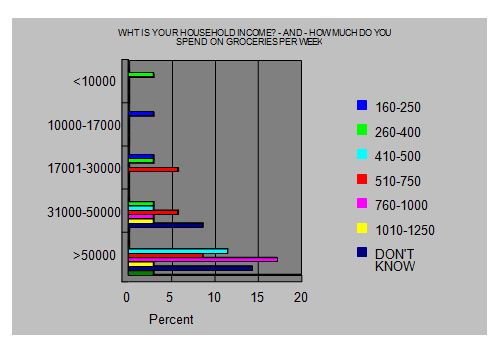
If we describe this curve then we can see the following things these are as follows:
- Almost 22% people spend more than 1250 taka in a week at supermarket and there income range is more than 50000 taka in a month.
- Almost 25% people spend in between 760-1000 in a week at supermarket and there income is also in between 31000-50000.
- Almost 18% people spend in between 510-750 in a week at supermarket and there income is also in between 17001-30000.
- Almost 14% people spend in between 410-500 in a week at supermarket and there income is also in between 10000-17000 taka.
FREQUENCY
WHAT IS YOUR GENDER?
Frequency | Valid Percent | ||
| Valid | Male | 15 | 43.O% |
| Female | 20 | 57.O% | |
| Total | 35 | 100.0% | |
| Missing | System | 0 | |
| Total | 35 | ||
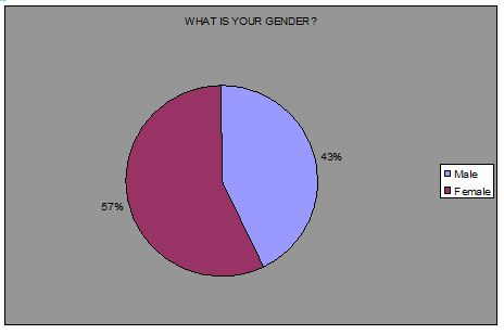
Comment:
Most of the customers those who go to the supermarket are female.
WHAT IS YOUR AGE?
Frequency | Valid Percent | ||
| Valid | 18-24 | 1 | 2.9% |
| 25-29 | 1 | 2.9% | |
| 30-34 | 7 | 20.0% | |
| 35-39 | 9 | 25.7% | |
| 40-44 | 11 | 31.4% | |
| 45-54 | 4 | 11.45 | |
| 55-64 | 2 | 5.75% | |
| Total | 35 | 100.0% | |
| Missing | System | 0 | 0 |
| Total | 35 | ||
z
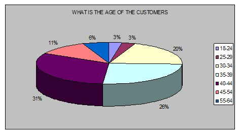
Comment:
People who are belonging the age in between 40-44 they are major customers of supermarket.
HOW MUCH DO YOU SPEND ON GROCERIES PER WEEK?
Frequency | Valid Percent | ||
| Valid | 10000-70000 | 2 | 5.7% |
| 17001-30000 | 4 | 11.5% | |
| 31000-50000 | 11 | 31.4% | |
| 51000+ | 18 | 51.4% | |
| Total | 35 | 100.0% | |
| Missing | System | 0 | 0 |
| Total | 35 | ||
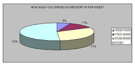
Comment:
People whose income is more than 51000 BDT normally they visit more in supermarket.
WHAT IS YOUR MARITAL STATUS?
Frequency | Valid Percent | ||
| Valid | Married | 29 | 82.8% |
| Single | 3 | 8.6% | |
| divorced | 3 | 8.6% | |
| Total | 35 | 100.0% | |
| Missing | System | 0 | |
| Total | 35 | ||
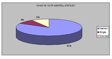
Comment:
We can see that the 82% of supermarket customers are married. It means married people most frequently visit the supermarket.
WHAT IS YOUR AVERAGE WEEKLY EXPENDITURE ON BOTH SUPERMARKETS AND SHOPS
Frequency | Valid Percent | ||
| Valid | 510-750 | 5 | 14.3% |
| 760-1000 | 7 | 20.0% | |
| 1010-1250 | 11 | 31.4% | |
| 1250+ | 12 | 34.3% | |
| Total | 35 | 100.0% | |
| Missing | System | 0 | 0 |
| Total | 35 | ||
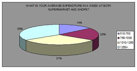
Comment:
Most of the supermarket customers spend more than 1250 BDT in a week at supermarket and shops.
WHAT IS YOUR AVERAGER WEEKLY EXPENDITURE ON SUPERMARKET?
Frequency | Valid Percent | ||
| Valid | 160-250 | 2 | 5.7% |
| 260-400 | 4 | 11.4% | |
| 410-500 | 10 | 28.6% | |
| 510-750 | 9 | 25.7% | |
| 760-1000 | 5 | 14.3% | |
| 1010-1250 | 2 | 5.7% | |
| 1250+ | 3 | 8.6% | |
| Total | 35 | 100.0% | |
| Missing | System | 0 | 0 |
| Total | 35 | ||
Comment: Most of the people spend in between 1010-1250 in a week at supermarket.
FREQUENCY OF THE GROCERY SHOPPING?
Frequency | Valid Percent | ||
| Valid | MORE THAN ONCE A WEEK | 4 | 11.4% |
| WEEKLY | 18 | 51.4% | |
| FORTNIGHTLY | 12 | 34.3% | |
| MONTHLY | 1 | 2.9% | |
| Total | 35 | 100.0% | |
| Missing | System | 0 | 0 |
| Total | 35 | ||
Comment: Most of the people go to supermarket in a weekly basis for their shopping.
IN WHICH SUPERMARKET YOU VISIT MOST FREQUENTLY?
Frequency | Valid Percent | ||
| Valid | NANDAN | 7 | 20.0% |
| AGORA | 10 | 28.6% | |
| PQS | 8 | 22.9% | |
| MEENABAZAR | 9 | 25.6% | |
| ALMAS | 1 | 2.9% | |
| Total | 35 | 100.0% | |
| Missing | System | 0 | |
| Total | 35 | ||
Comment: people use more Agora for their grocery shopping compare to the others SM.
WHAT TYPES OF PRODUCTS YOU USUALLY BUY FROM SUPERMARKRT?
Frequency | Valid Percent | ||
| Valid | CONFECTIONARY | 15 | 42.9% |
| READY PREPARED MEALS | 13 | 37.1% | |
| DIY PRODUCTS | 2 | 5.7% | |
| TOILETRIS | 5 | 14.3% | |
| Total | 35 | 100.0% | |
| Missing | System | 0 | |
| Total | 35 | ||
Comment: people purchase more the confectionary items from the supermarket.
IN WHICH SUPERMARKET YOU NORMALLY VISIT FOR YOUR GROCERIES?
Frequency | Valid Percent | ||
| Valid | NANDAN | 5 | 14.3 |
| AGORA | 11 | 31.4 | |
| PQS | 8 | 22.9 | |
| MEENABAZAR | 9 | 25.7 | |
| ALMAS | 2 | 5.7 | |
| Total | 35 | 100.0 | |
| Missing | System | 0 | 0 |
| Total | 35 | ||
Comment: Many people use Agora for their top up shopping.
HOW MUCH YOU SPEN FOR YOUR TOP UP EXPENDITURE?
Frequency | Valid Percent | ||
| Valid | 160-250 | 7 | 20.0% |
| 260-400 | 6 | 17.1% | |
| 410-500 | 14 | 40.0% | |
| 501-750 | 7 | 20.0% | |
| 750+ | 1 | 2.9% | |
| Total | 35 | 100.0% | |
| Missing | System | 0 |
Comment: people spend in between 410-500 BDT for their top up shopping in week.
WHAT TYPES OF TRANSPORT YOU NORMALLY USE TO GO THE SUPERMARKET?
Frequency | Valid Percent | ||
| Valid | CAR | 21 | 60.0% |
| ON FOOT | 5 | 14.3% | |
| RICKSHAW | 9 | 25.7% | |
| Total | 35 | 100.0% | |
| Missing | System | 0 | |
| Total | 35 | ||
Comment: Almost 60% of the supermarket customers use car to go to supermarket.
WHAT IS THE TRAVEL DISTANCE OF YOUR REGULAR VISITD SUPERMARKET?
Frequency | Valid Percent | ||
| Valid | >1MILE | 20 | 57.1% |
| 2MILES | 13 | 37.2% | |
| 3MILES | 2 | 5.7% | |
| Total | 35 | 100.0% | |
| Missing | System | 0 | |
| Total | 35 | ||
Comment: Most of the supermarket customers travel distance is within one mile.
WHAT IS THE APPROXIMATE TRAVEL TIME TO REACH THE SUPERMARKET
Frequency | Valid Percent | ||
| Valid | 5 MINUTES | 1 | 2.9% |
| 6-10 MINUTES | 10 | 28.6% | |
| 11-20 MINUTES | 17 | 48.6% | |
| 21-30 MINUTES | 6 | 17.0% | |
| 31-60 MINUTES | 1 | 2.9% | |
| Total | 35 | 100.0% | |
| Missing | System | 0 | |
| Total | 35 | ||
Comment: Most of the people require at least 11-20 minutes going to supermarket.
WHAT IS YOUR VEST ALTERNATIVE TO ACCOMPLISH OF YOUR SHOPPING?
Frequency | Valid Percent | ||
| Valid | NANDAN | 10 | 28.6% |
| AGORA | 10 | 28.6% | |
| PQS | 5 | 14.3% | |
| MINA BAZAR | 5 | 14.3% | |
| ALMAS | 3 | 8.6% | |
| SHOP N SAVE | 2 | 5.7% | |
| Total | 35 | 100.0% | |
| Missing | System | 0 | |
| Total | 35 | ||
Comment: Most of the people say that their best alternative is either Agora or Nandan.
WHAT TYPES OF BRAD YOU LIKE WHEN PURCHASR YOUR GROCERIES
Frequency | Valid Percent | ||
| Valid | MAINLY SUPERMARKET OWNED BRAND | 3 | 8.6% |
| MAINLY NON-SUPERMARKET BRANDS | 17 | 48.6% | |
| A MIX OF BOTH | 13 | 37.1% | |
| DONT KNOW | 2 | 5.7% | |
| Total | 35 | 100.0% | |
| Missing | System | 0 | |
| Total | 36 | ||
Comment: Most of the people purchase the non supermarket brand from the supermarket.
WHICH TYPE OF PEOOFFER YOU LIKE MOST FROM YOUR SUPERMARKET?
Frequency | Valid Percent | ||
| Valid | 2 FOR THE PRICE OF 1 | 8 | 22.8% |
| BUY 1 ITEM GET 1 FREE | 12 | 34.3% | |
| PRICE REDUCTION COUPON | 8 | 22.9% | |
| REFUND PROMISE | 7 | 20.0% | |
| Total | 35 | 100.0% | |
| Missing | System | 0 |
Comment: Most of the customers of supermarket like the promotional offer which is buy one item and gets one free.
REGRESSION
IV = WHAT IS YOUR AGE?
Mean = 3.300
Standard Deviation = 1.84
DV = WHT IS YOUR HOUSEHOLD INCOME?
Mean = 2.450
Standard Deviation = 4.382
Goodness of Fit
Mean of Residuals = 0.000
Standard Deviation of Residuals = 0.983
Mean Absolute Percent Error = 25.783%
Mean Percent Error = -1O.350%
Mean Square Error = 0.842
Regression Statistics data
Valid Cases = 35
Missing Cases = 0
Correlation Coefficient = 0.195
Degrees of Freedom = 32
Adjusted R-Squared = 0.012
Standard Error of the Estimate = 0.987
Regression Coefficients chart
Coefficient Est. Std. Error T-Value Significance
Intercept 3.976 0.431 12.201 0.0000
Slope 0.121 0.086 1.133 0.3426
Table of pragmatic Data, Predicted Data, and % of Error
Rec IV DV Predicted Residual Std. Resid. % Error – 95% CI + 95% CI
1 3 1 5 -4 -4.267 -315.0 4 5
2 4 4 3 0 -0.316 -11.1 4 5
3 1 5 3 1 0.968 17.6 4 5
4 4 5 4 1 0.613 11.9 4 5
5 1 3 4 -1 -1.097 -35.6 4 5
6 1 5 4 1 0.957 18.6 4 5
7 1 5 4 1 0.957 18.6 4 5
8 1 5 4 1 0.957 18.6 4 5
9 3 4 4 0 -0.300 -7.3 4 5
10 3 4 4 0 -0.300 -7.3 4 5
11 5 5 5 0 0.498 9.7 4 5
12 3 4 4 0 -0.300 -7.3 4 5
13 6 5 5 0 0.383 7.5 4 5
14 5 5 5 0 0.498 9.7 4 5
15 1 5 4 1 0.957 18.6 4 5
16 3 5 4 1 0.727 14.2 4 5
17 3 4 4 0 -0.300 -7.3 4 5
18 6 5 5 0 0.383 7.5 4 5
19 3 5 4 1 0.727 14.2 4 5
20 2 5 4 1 0.842 16.4 4 5
21 2 4 4 0 -0.185 -4.5 4 5
22 2 3 4 -1 -1.212 -39.3 4 5
Rec IV DV Predicted Residual Std. Resid. % Error – 95% CI + 95% CI
23 2 3 4 -1 -1.212 -39.3 4 5
24 5 5 5 0 0.498 9.7 4 5
25 1 5 4 1 0.957 18.6 4 5
26 1 5 4 1 0.957 18.6 4 5
27 2 2 4 -2 -2.239 -109.0 4 5
28 5 4 5 -1 -0.529 -12.9 4 5
29 6 4 5 -1 -0.644 -15.7 4 5
30 7 5 5 0 0.268 5.2 4 6
31 4 4 4 0 -0.415 -10.1 4 5
32 4 5 4 1 0.613 11.9 4 5
33 5 5 5 0 0.498 9.7 4 5
34 4 3 4 -1 -1.442 -46.8 4 5
35 4 5 4 1 0.613 11.9 4 5
Comment:
Customer’s household income largely depends on the age of the customers.
IV = WHT IS YOUR HOUSEHOLD INCOME?
Mean = 4.268
Standard Deviation = 0.986
DV = HOW MUCH DO YOU SPEND ON GROCERY ITEAMS IN EVERY WEEK?
Mean = 3.632
Standard Deviation = 6.798
Goodness of Fit
Mean of Residuals = 0.000
Standard Deviation of Residuals = 0.969
Mean Absolute Percent Error = 13.750%
Mean Percent Error = -2.243%
Mean Square Error = 0.976
Regression Statistics
Valid Cases = 35
Missing Cases = 0
Correlation Coefficient = 0.569
Degrees of Freedom = 33
Adjusted R-Squared = 0.272
Standard Error of the Estimate = 1.009
Regression Coefficients chart
Coefficient Est. Std. Error T-Value Significance
Intercept 4.433 0.760 5.686 0.0000
Slope 0.763 0.273 2.507 0.0010
Table of pragmatic Data, Predicted Data, and Error
Rec IV DV Predicted Residual Std. Resid. % Error – 95% CI + 95% CI
1 1 4 5 -1 -1.012 -25.1 4 6
2 4 8 7 1 1.119 13.9 7 7
3 5 8 8 0 0.487 6.0 7 8
4 5 9 8 1 1.494 16.5 7 8
5 3 7 6 1 0.745 10.6 6 7
6 5 7 8 -1 -0.520 -7.4 7 8
7 5 7 8 -1 -0.520 -7.4 7 8
8 5 5 8 -3 -2.534 -50.3 7 8
9 4 6 7 -1 -0.895 -14.8 7 7
10 4 6 7 -1 -0.895 -14.8 7 7
11 5 7 8 -1 -0.520 -7.4 7 8
12 4 6 7 -1 -0.895 -14.8 7 7
13 5 8 8 0 0.487 6.0 7 8
14 5 5 8 -3 -2.534 -50.3 7 8
15 5 8 8 0 0.487 6.0 7 8
16 5 8 8 0 0.487 6.0 7 8
17 4 8 7 1 1.119 13.9 7 7
18 5 8 8 0 0.487 6.0 7 8
19 5 7 8 -1 -0.520 -7.4 7 8
20 5 8 8 0 0.487 6.0 7 8
21 4 5 7 -2 -1.902 -37.8 7 7
22 3 7 6 1 0.745 10.6 6 7
Rec IV DV Predicted Residual Std. Resid. % Error – 95% CI + 95% CI
23 3 7 6 1 0.745 10.6 6 7
24 5 8 8 0 0.487 6.0 7 8
25 5 8 8 0 0.487 6.0 7 8
26 5 7 8 -1 -0.520 -7.4 7 8
27 2 5 6 -1 -0.637 -12.7 5 7
28 4 8 7 1 1.119 13.9 7 7
29 4 8 7 1 1.119 13.9 7 7
30 5 8 8 0 0.487 6.0 7 8
31 4 7 7 0 0.112 1.6 7 7
32 5 8 8 0 0.487 6.0 7 8
33 5 7 8 -1 -0.520 -7.4 7 8
34 3 7 6 1 0.745 10.6 6 7
35 5 8 8 0 0.487 6.0 7 8
Comment:
Customers spend on the grocery items from both supermarket and shops depend on the customers hose hold income.
IV = WHT IS YOUR HOUSEHOLD INCOME?
Mean = 4.314
Standard Deviation = 0.993
DV = HOW MUCH DO YOU SPEND ON GROCERY ITEAMS PER WEEK AT SUPERMARKETS?
Mean =
Standard Deviation = 5.711
Goodness of Fit
Mean of Residuals = 0.000
Standard Deviation of Residuals = 1.641
Mean Absolute Percent Error = 29.154%
Mean Percent Error = -10.308%
Mean Square Error = 2.615
Regression Statistics
Valid Cases = 35
Missing Cases = 0
Correlation Coefficient = 0.513
Degrees of Freedom = 33
Adjusted R-Squared = 0.240
Standard Error of the Estimate = 1.665
Regression Coefficients Table
Coefficient Est. Std. Error T-Value Significance
Intercept 1.373 1.272 1.079 0.2883
Slope 0.986 0.288 3.430 0.0016
Table of pragmatic Data, Predicted Data, and Error
Rec IV DV Predicted Residual Std. Resid. % Error – 95% CI + 95% CI
1 1 3 2 1 0.390 21.4 0 4
2 4 7 5 2 1.025 24.0 5 6
3 5 5 6 -1 -0.795 -26.1 6 7
4 5 9 6 3 1.643 29.9 6 7
5 3 5 4 1 0.407 13.4 3 5
6 5 4 6 -2 -1.405 -57.6 6 7
7 5 4 6 -2 -1.405 -57.6 6 7
8 5 5 6 -1 -0.795 -26.1 6 7
9 4 3 5 -2 -1.413 -77.3 5 6
10 4 4 5 -1 -0.804 -33.0 5 6
11 5 4 6 -2 -1.405 -57.6 6 7
12 4 6 5 1 0.415 11.4 5 6
13 5 8 6 2 1.033 21.2 6 7
14 5 4 6 -2 -1.405 -57.6 6 7
15 5 6 6 0 -0.186 -5.1 6 7
16 5 6 6 0 -0.186 -5.1 6 7
17 4 8 5 3 1.634 33.5 5 6
18 5 7 6 1 0.424 9.9 6 7
19 5 6 6 0 -0.186 -5.1 6 7
20 5 8 6 2 1.033 21.2 6 7
21 4 5 5 0 -0.194 -6.4 5 6
22 3 2 4 -2 -1.421 -116.6 3 5
Rec IV DV Predicted Residual Std. Resid. % Error – 95% CI + 95% CI
23 3 5 4 1 0.407 13.4 3 5
24 5 6 6 0 -0.186 -5.1 6 7
25 5 8 6 2 1.033 21.2 6 7
26 5 5 6 -1 -0.795 -26.1 6 7
27 2 2 3 -1 -0.820 -67.3 2 5
28 4 8 5 3 1.634 33.5 5 6
29 4 8 5 3 1.634 33.5 5 6
30 5 8 6 2 1.033 21.2 6 7
31 4 5 5 0 -0.194 -6.4 5 6
32 5 6 6 0 -0.186 -5.1 6 7
33 5 6 6 0 -0.186 -5.1 6 7
34 3 3 4 -1 -0.812 -44.4 3 5
35 5 8 6 2 1.033 21.2 6 7
Comment:
People’s expenditure on grocery items at supermarket largely depends on the household income.
IV = WHAT IS THE APPROXIMATE TRAVEL TIME TO REACH THE SUPER MARKET?
Mean = 2.530
Standard Deviation = 1.237
DV = WHAT IS THE APPROXIMATE TRAVEL DISTANCE OF THE SUPER MARKET FROM YOUR HOME?
Mean = 2.672
Standard Deviation = 1.474
Goodness of Fit
Mean of Residuals = 0.000
Standard Deviation of Residuals = 0.650
Mean Absolute Percent Error = 35.235%
Mean Percent Error = -12.001%
Mean Square Error = 0.432
Regression Statistics
Valid Cases = 35
Missing Cases = 0
Correlation Coefficient = 0.817
Degrees of Freedom = 33
Adjusted R-Squared = 0.399
Standard Error of the Estimate = 0.757
Regression Coefficients Table
Coefficient Est. Std. Error T-Value Significance
Intercept 0.073 0.228 0.232 0.6948
Slope 0.659 0.078 4.402 0.0000
Table of pragmatic Data, Predicted Data, and Error
Rec IV DV Predicted Residual Std. Resid. % Error – 95% CI + 95% CI
1 2 1 1 0 -0.327 -24.8 1 2
2 1 1 1 0 0.444 33.8 0 1
3 2 1 1 0 -0.327 -24.8 1 2
4 1 1 1 0 0.444 33.8 0 1
5 4 2 2 0 -0.553 -21.0 2 3
6 6 4 4 0 0.536 10.2 3 4
7 6 4 4 0 0.536 10.2 3 4
8 3 2 2 0 0.218 8.3 2 2
9 1 1 1 0 0.444 33.8 0 1
10 1 1 1 0 0.444 33.8 0 1
11 2 2 1 1 0.989 37.6 1 2
12 2 1 1 0 -0.327 -24.8 1 2
13 3 1 2 -1 -1.098 -83.4 2 2
14 1 1 1 0 0.444 33.8 0 1
15 2 1 1 0 -0.327 -24.8 1 2
16 3 1 2 -1 -1.098 -83.4 2 2
17 2 1 1 0 -0.327 -24.8 1 2
18 5 3 3 0 -0.009 -0.2 2 4
19 1 1 1 0 0.444 33.8 0 1
20 2 1 1 0 -0.327 -24.8 1 2
21 4 2 2 0 -0.553 -21.0 2 3
22 2 1 1 0 -0.327 -24.8 1 2
Rec IV DV Predicted Residual Std. Resid. % Error – 95% CI + 95% CI
23 4 2 2 0 -0.553 -21.0 2 3
24 2 1 1 0 -0.327 -24.8 1 2
25 1 1 1 0 0.444 33.8 0 1
26 2 1 1 0 -0.327 -24.8 1 2
27 3 1 2 -1 -1.098 -83.4 2 2
28 3 1 2 -1 -1.098 -83.4 2 2
29 3 1 2 -1 -1.098 -83.4 2 2
30 3 1 2 -1 -1.098 -83.4 2 2
31 4 4 2 2 2.078 39.5 2 3
32 3 5 2 3 4.164 63.3 2 2
33 3 2 2 0 0.218 8.3 2 2
34 2 1 1 0 -0.327 -24.8 1 2
35 2 1 1 0 -0.327 -24.8 1 2
Comment:
The time needed to reach the supermarket largely depends on the distance of the supermarket from customer’s home.
DESCRIPTIVE
WHT IS YOUR HOUSEHOLD INCOME?
Minimum = 1
Maximum = 7
Mean = 5.13
Median = 6
Variance (Unbiased) = 0.97
Standard Deviation (Unbiased) = 0.97
Standard Error of the Mean = 0.15
95 Percent Confidence Interval around the Mean = 3.77 – 4.65
99 Percent Confidence Interval around the Mean = 2.98 – 4.85
4 Groups
1 = 4
2 = 5
3 = 5
Valid Cases = 35
Missing Cases = 0
Response Percent = 100.0%
HOW MUCH DO YOU SPEND ON GROCERIES PER WEEK AT SUPERMARKETS?
Minimum = 1
Maximum = 8
Mean = 4.52
Median = 6
Variance (Unbiased) = 3.54
Standard Deviation (Unbiased) = 1.92
Standard Error Of The Mean = 0.30
95 Percent Confidence Interval Around The Mean = 5.00 – 6.38
99 Percent Confidence Interval Around The Mean = 4.5 0 – 6.64
4 Groups
1 = 4
2 = 5.35
3 = 7.65
Valid Cases = 35
Missing Cases = 0
Response Percent = 100.0%
BREAK-DOWN
WHT IS YOUR HOUSEHOLD
INCOME? Mean SD N Pct.
For Entire Sample (Missing = 0) 4.254 .93 35 100.0%
HOW MUCH YOU
SPEND ON GROCERY ITEAMS PER
WEEK AT
SUPERMARKETS?
1=<150 0.00 0.00 0 0.0%
2=160-250 2.50 0.71 2 7.4%
3=260-400 2.67 1.53 3 11.1%
4=410-500 4.80 0.45 5 18.5%
5=510-750 4.14 0.90 7 25.9%
6=760-1000 4.86 0.38 7 25.9%
7=1010-1250 4.50 0.71 2 7.4%
9=DON’T KNOW 5.00 0.00 1 3.8%
Comments:
If we analyze the above data then we can see that the people don’t spend less then 150 in a week at supermarket. Besides, we can see that the people usually spend in between 510-750 and 760-1000 taka at supermarket. In addition people also spend more than 1250 in a week at supermarket. This thing happens because customer expenditure level changes with the change of their income. But we can state that most people purchase their grocery items with in 1000 taka from the supermarket.
DESCRIMINATE
Dependent Variable: WHAT IS
WHAT IS YOUR GENDER?
Group Code Group Name N Prior Prob.
1 MALE 15 0.429
2 FEMALE 20 0.571
Descriptive Statistics for All Groups
Variable Mean SD
V2 WHAT IS YOUR AGE? 3.300 1.832
V3 WHT IS YOUR HOUSEHOLD INCOME? 5.325 0.899
Number of Valid Cases = 35
Number of Missing Cases = 0
Response Percent = 100.0 %
Within Groups Correlation Matrix
| V2 | ||
| V2 | r | 0.082 |
| p | 0.732 |
Step1
Variable V3 Entered
Lambda =0.832 F(1,34)=9.531, p=0.008
Var. F-to-Remove F-to-Enter
V2 1.987
V3 9.724
Stepwise Discriminate Function Analysis Summary
Step Variable Wilkes F-Value to
No. Entered Removed Lambda Enter/Remove No. of IVs
1 V3 0.832 9.724 1
Group Classification Function Coefficients
| 1 | 2 | |
| V3 | 5.321 | 8.009 |
| Const. | -9.753 | -13.321 |
Incorrect Classifications:
- Record 4 from group 1 was incorrectly classified in group 2
- Record 5 from group 1 was incorrectly classified in group 2
- Record 6 from group 1 was incorrectly classified in group 2
- Record 8 from group 1 was incorrectly classified in group 2
- Record 12 from group 1 was incorrectly classified in group 2
- Record 13 from group 1 was incorrectly classified in group 2
- Record 20 from group 1 was incorrectly classified in group 2
- Record 22 from group 1 was incorrectly classified in group 2
- Record 30 from group 1 was incorrectly classified in group 2
Classification Matrix (Number of cases classified in each group)
| Group | % Correct | 1 | 2 |
| 1 | 42.0 | 7 | 1O |
| 2 | 100.0 | 0 | 20 |
| Total | 76.4 | 7 | 30 |
Canonical Variable Summary
Eigenvalue Proportion Cumulative Canonical Correlation
CANO1 0.362 100.00 100.00 0.533
Total variance = 0.355
Canonical Variable Coefficients
| Variable | CANO1 |
| V3 | 0.000 |
Canonical Variables Evaluated at Group Means
| Group | CANO1 |
| 1 | 0.642 |
| 2 | -0.382 |
KEY FINDINGS:
- People who earn more than 50000 taka they are the key customers of the supermarket because of their high purchasing power.
- Young people, especially young married women purchase more from the supermarket because they immensely like the hassle free environment for shopping.
- Household income doesn’t have any enormous impact on choosing the supermarket.
- Convenient location of supermarket, variety of products, nice environment, reasonable price, and hassle free payment system are some crucial factors for choosing the best supermarket by the customers.
- People normally purchase more the confectionary items from the supermarket then the other products.
- Too much distance of a supermarket is also a reason for neglecting by the customers.
- People accomplish most of their top up shopping from the supermarkets.
- Supermarket own brand product sometimes attract the potential customers towards the supermarkets.
- People usually like the buy one and get one free type promotional offer from the supermarkets but they become happier if they get the reasonable price products from supermarket.
Recommendations:
- Supermarket should promote themselves more and more through media because in our country we see hardly any ad on supermarket in TV or in other media.
- Supermarket should be more geographically diverse, especially in every big cities of Bangladesh.
- There is a common complain against the supermarkets that they charge too much price for their products. So, supermarket should design their pricing strategy such a way so that it doesn’t hamper their profit and more importantly their customers.
- Since people willing to pay some extra price 1-2% for the nice environment so, supermarkets should improve their outlet environment considering their customers.
- Supermarket should include more variety of products with there current product line so that they can easily attract the customers.
- They can offer special discount on some products targeting specific group of customers which can boost up their sales.
- They can offer home delivery service of their goods for their customers like- MacDonald’s which may help to explore their business a great deal because urban people are now so busy and they don’t have enough time for conducting their shopping.
- They can open a special corner for the middle class people those income ranges is in between 8000-15000 BDT then they can easily boost up their sales.
- Supermarkets should place the effective, efficient, trained, and cooperative sales person who can easily satisfy the customers by his/her service.