P1: Identify and classify different types of cost:
definaion of prime cost, production cost, admin cost and selling & distribution cost.
Prime cost
Direct cost of labour and material for producing a product without the overhead is called prime cost.
Production cost
Production cost is the expenses consist of direct materials, direct labour, and factory overhead which are closely related with the manufacturing activities of the company, admin cost
Expense incurred in controlling and directing an organization, but this is not any part of marketing, or production operations.
selling & distribution cost
Expenses made for marketing and distribution of a product.
Cost Sheet
Raw materials 118830
Factory wages 117315
Prime cost: 236145
Rent & rates of company 16460
Factory power 3825
Factory heat and light 1185
Depreciation on factory plant and machinery 3715
25185
Production cost: 261330
Salary paid to office staff 4095
Depriciation on office computer equipment 2425
Admin cost: 6520
Advertising 11085
Sales staff salary 4095
Cost of trade exhibition 1500
Selling and dis: cost: 16680
Total cost 284530
P2: Explain the need for, and operation of, different costing methods:
An accountant
A construction company
Contract Costing: Contract costing is applied for contract work like construction of dam building civil engineering contract etc. each contract or job is treated as separate cost unit for the cost ascertainment and control.
A hotel
An airline company
Standard cost is the company’s fixed costs over a given period of time to the items produced during that period, and recording the result as the total cost of production.
For an airline company It is the best.
A baker
Batch Costing: A batch is a group of identical products. Under batch costing a batch of similar products is treated as a separate unit for the purpose of ascertaining cost. The total costs of a batch is divided by the total number of units in a batch to arrive at the costs per unit.
P3: Calculate costs using appropriate techniques: Work in progress valuation
| Work in Progess | ||||||||||
| cost | Completed toys | toys | % completed | Equvelent unit | Total Equvelent unit | Cost per toys | WIP valuation | Completed with valuation | Total cost per production | |
| Direct materials | 11500 | 20000 | 5000 | 100% | 5000 | 25000 | 0.46 | 2300 | 9200 | 11500 |
| Direct Labour | 9000 | 20000 | 5000 | 50% | 2500 | 22500 | 0.4 | 1000 | 8000 | 9000 |
| Production O/D | 18000 | 20000 | 5000 | 50% | 2500 | 22500 | 0.8 | 2000 | 16000 | 18000 |
| Total | 38500 | 1.66 | 5300 | 33200 | 38500 | |||||
Cost per toy is 1.66
Valuation in progress is 5300
P4: Collect, analyse and present data using appropriate techniques:
Analysis of data is a process of inspecting, cleaning, transforming, and modeling data with the goal of highlighting useful information, suggesting conclusions, and supporting decision making. Data analysis has multiple facets and approaches, encompassing diverse techniques under a variety of names, in different business, science, and social science domains.
Data mining is a particular data analysis technique that focuses on modeling and knowledge discovery for predictive rather than purely descriptive purposes. Business intelligence covers data analysis that relies heavily on aggregation, focusing on business information. In statistical applications, some people divide data analysis into descriptive statistics, exploratory data analysis, and confirmatory data analysis. EDA focuses on discovering new features in the data and CDA on confirming or falsifying existing hypotheses. Predictive analytics focuses on application of statistical or structural models for predictive forecasting or classification, while text analytics applies statistical, linguistic, and structural techniques to extract and classify information from textual sources, a species of unstructured data. All are varieties of data analysis.
Data integration is a precursor to data analysis, and data analysis is closely linked to data visualization and data dissemination. The term data analysis is sometimes used as a synonym for data modeling, which is unrelated to the subject of this article.
The process of data analysis
Data analysis is a process, within which several phases can be distinguished:[1]
- Data cleaning
- Initial data analysis (assessment of data quality)
- Main data analysis (answer the original research question)
- Final data analysis (necessary additional analyses and report)
Data cleaning
Data cleaning is an important procedure during which the data are inspected, and erroneous data are -if necessary, preferable, and possible- corrected. Data cleaning can be done during the stage of data entry. If this is done, it is important that no subjective decisions are made. The guiding principle provided by Adèr (ref) is: during subsequent manipulations of the data, information should always be cumulatively retrievable. In other words, it should always be possible to undo any data set alterations. Therefore, it is important not to throw information away at any stage in the data cleaning phase. All information should be saved (i.e., when altering variables, both the original values and the new values should be kept, either in a duplicate dataset or under a different variable name), and all alterations to the data set should carefully and clearly documented, for instance in a syntax or a log.[2]
Initial data analysis
The most important distinction between the initial data analysis phase and the main analysis phase, is that during initial data analysis one refrains from any analysis that are aimed at answering the original research question. The initial data analysis phase is guided by the following four questions:[3]
Quality of data
The quality of the data should be checked as early as possible. Data quality can be assessed in several ways, using different types of analyses: frequency counts, descriptive statistics (mean, standard deviation, median), normality (skewness, kurtosis, frequency histograms, normal probability plots), associations (correlations, scatter plots).
Other initial data quality checks are:
- Checks on data cleaning: have decisions influenced the distribution of the variables? The distribution of the variables before data cleaning is compared to the distribution of the variables after data cleaning to see whether data cleaning has had unwanted effects on the data.
- Analysis of missing observations: are there many missing values, and are the values missing at random? The missing observations in the data are analyzed to see whether more than 25% of the values are missing, whether they are missing at random (MAR), and whether some form of imputation (statistics) is needed.
- Analysis of extreme observations: outlying observations in the data are analyzed to see if they seem to disturb the distribution.
- Comparison and correction of differences in coding schemes: variables are compared with coding schemes of variables external to the data set, and possibly corrected if coding schemes are not comparable.
The choice of analyses to assess the data quality during the initial data analysis phase depends on the analyses that will be conducted in the main analysis phase.[4] by philip kotler
Quality of measurements
The quality of the measurement instruments should only be checked during the initial data analysis phase when this is not the focus or research question of the study. One should check whether structure of measurement instruments corresponds to structure reported in the literature.
There are two ways to assess measurement quality:
- Confirmatory factor analysis
- Analysis of homogeneity (internal consistency), which gives an indication of the reliability of a measurement instrument, i.e., whether all items fit into a unidimensional scale. During this analysis, one inspects the variances of the items and the scales, the Cronbach’s α of the scales, and the change in the Cronbach’s alpha when an item would be deleted from a scale.[5]
Initial transformations
After assessing the quality of the data and of the measurements, one might decide to impute missing data, or to perform initial transformations of one or more variables, although this can also be done during the main analysis phase.[6]
Possible transformations of variables are:[7]
- Square root transformation (if the distribution differs moderately from normal)
- Log-transformation (if the distribution differs substantially from normal)
- Inverse transformation (if the distribution differs severely from normal)
- Make categorical (ordinal / dichotomous) (if the distribution differs severely from normal, and no transformations help)
Did the implementation of the study fulfill the intentions of the research design?
One should check the success of the randomization procedure, for instance by checking whether background and substantive variables are equally distributed within and across groups.
If the study did not need and/or use a randomization procedure, one should check the success of the non-random sampling, for instance by checking whether all subgroups of the population of interest are represented in sample.
Other possible data distortions that should be checked are:
- dropout (this should be identified during the initial data analysis phase)
- Item nonresponse (whether this is random or not should be assessed during the initial data analysis phase)
- Treatment quality (using manipulation checks).[8]
Characteristics of data sample
In any report or article, the structure of the sample must be accurately described. It is especially important to exactly determine the structure of the sample (and specifically the size of the subgroups) when subgroup analyses will be performed during the main analysis phase.
The characteristics of the data sample can be assessed by looking at:
- Basic statistics of important variables
- Scatter plots
- Correlations
- Cross-tabulations[9]
Final stage of the initial data analysis
During the final stage, the findings of the initial data analysis are documented, and necessary, preferable, and possible corrective actions are taken.
Also, the original plan for the main data analyses can and should be specified in more detail and/or rewritten.
In order to do this, several decisions about the main data analyses can and should be made:
- In the case of non-normals: should one transform variables; make variables categorical (ordinal/dichotomous); adapt the analysis method?
- In the case of missing data: should one neglect or impute the missing data; which imputation technique should be used?
- In the case of outliers: should one use robust analysis techniques?
- In case items do not fit the scale: should one adapt the measurement instrument by omitting items, or rather ensure comparability with other (uses of the) measurement instrument(s)?
- In the case of (too) small subgroups: should one drop the hypothesis about inter-group differences, or use small sample techniques, like exact tests or bootstrapping?
- In case the randomization procedure seems to be defective: can and should one calculate propensity scores and include them as covariates in the main analyses?[10]
Analyses
Several analyses can be used during the initial data analysis phase:[11]
- Univariate statistics
- Bivariate associations (correlations)
- Graphical techniques (scatter plots)
It is important to take the measurement levels of the variables into account for the analyses, as special statistical techniques are available for each level:[12]
- Nominal and ordinal variables
- Frequency counts (numbers and percentages)
- Associations
- circumambulations (crosstabulations)
- hierarchical loglinear analysis (restricted to a maximum of 8 variables)
- loglinear analysis (to identify relevant/important variables and possible confounders)
- Exact tests or bootstrapping (in case subgroups are small)
- Computation of new variables
- Continuous variables
- Distribution
- Statistics (M, SD, variance, skewness, kurtosis)
- Stem-and-leaf displays
- Box plots
- Distribution
P5: Prepare and analyse routine cost reports:
Exe wye
Production in a week 50000 50000
Production in abatch 10000 1000
Batch required 5 50
Total setup cost = set up cost x total number of batch
= 250 x 55
= 13750
Total quality inspection = quality inspection x total number of batch
= 150 x 55
= 8250
| Labour | ABC | ||||
| Batch er cost | Exe | Wye | Exe | wye | |
| Set up | |||||
cost25068756875125012500Quality inspection150412541257507500 1100011000200020000total2200022000
P6: Calculate and evaluate indicators of productivity, efficiency and effectiveness:
1. Labour Productivity (output per = output / no of employee)
A = 320000/ 120 B = 400000/ 130 C = 325000/ 135 D = 1045000/ 385
= 2666.67 = 3076.92 = 2407.41 = 2714.29
2. Capital productivity (output per capital employed = output / capital employed)
A = 320000/ 1300 B = 400000/ 1250 C = 325000/ 1250 D = 1045000/ 3800
= 246.15 = 320 = 260 = 275
3. Machine productivity ( output per machine = output / machine hours for paid)
A = 320000/ 54720 B = 400000/ 62400 C = 325000/ 69660
= 5.85 = 6.41 = 4.66
D = 1045000/ 186780
= 5.59
4. Efficiency = (actual output / standard output X 100%)
A = 320000 / 300000 X 100 B = 400000 / 360000 X 100
= 106.6% = 111.1%
C = 325000 / 375000 X 100 D = 1045000 / 1035000 X 100
= 86.6% = 100.9%
5. Effectiveness = (Actual hour work / standard hour work X 100)
A = 54720 /55200 X 100 B = 62400 / 63000 X 100
= 99.1% = 99.0%
C = 69660 / 75000 X 100 D = 186780 / 193200 X 100
= 92.8% = 96.6%
P7: Explain the principles of quality and value, and identify potential improvements:
All else being equal, good quality customer service gives the edge over competitors. Regardless of industry, here are the 9 key principals of good customer service that always make business sense.
1. Attracting new customers costs more than retaining existing customers
A satisfied customer stays with a company longer, spends more and may deepen the relationship. For example a happy credit card customer may enlist the company’s financial services and later take travel insurance.
This is an easy “sell”, compared with direct marketing campaigns, television advertisements and other sophisticated and expensive approaches to attract new customers.
2. Customer service costs real money
Real costs are associated with providing customer service and companies spend in line with a customer’s value. If you are a high value customer or have the potential of being high value, you will be serviced more carefully.
Companies reduce the cost of customer service by using telephone voice response systems, outsourcing call centers to cheaper locations, and self-servicing on the internet. However, companies risk alienating customers through providing an impersonal service.
Some internet banking companies are bucking the trend by charging customers to contact them. In exchange, customers receive better interest rates due to reduced overheads and are satisfied with that.
3. Understand your customers’ needs and meet them
How can you meet your customers’ needs, if you don’t know them? To understand your customer’s needs, just listen to the “voice of the customer” and take action accordingly.
Customer listening can be done in many ways, for example feedback forms, mystery shopping, and satisfaction surveys. Some companies involve senior employees in customer listening to ensure decisions benefit the customer as much as the company.
4. Good process and product design is important
Good quality customer service is only one factor in meeting customer needs. Well designed products and processes will meet customers’ needs more often. Quality movements, such as Six Sigma, consider the “cost of quality” resulting from broken processes or products. Is it better to service the customer well than to eradicate the reason for them to contact you in the first instance?
5. Customer service must be consistent
Customers expect consistent quality of customer service; with a similar, familiar look and feel whenever and however they contact the company.
Say you visit an expensive hairdressing salon and receive a friendly welcome, a drink and a great haircut. You are out of town and visit the same hairdressing chain and get no friendly welcome, no drink and a great hair-cut. Are you a satisfied customer who will use that chain again? Probably not, as you did not receive the same customer service – which is more than a good hair-cut.
6. Employees are customers too
The quality management movement brought the concept of internal and external customers. Traditionally the focus was on external customers with little thought given to how internal departments interacted. Improving relationships with internal customers and suppliers assists delivery of better customer service to external customers, through reduced lead-times, increased quality and better communication.
The “Service-Profit Chain” model developed by Harvard University emphasizes the circular relationship between employees, customers and shareholders. Under-staffed, under-trained employees will not deliver good quality customer service, driving customers away. Equal effort must be made in attracting, motivating and retaining employees as is made for customers, ultimately delivering improved shareholder returns. Better shareholder returns mean more money is available to invest in employees and so the circle continues.
7. Open all communications channels
The customer wants to contact you in many ways – face to face, by mail, phone, fax, and email – and will expect all of these communication channels to be open and easily inter-mingled.
This presents a technical challenge, as it requires an integrated, streamlined solution providing the employee with the information they need to effectively service the customer.
8. Every customer contact is a chance to shine
If a customer contact concerns a broken process, then empowered employees will be able to resolve the complaint swiftly, possibly enhancing the customer’s perception of the company. Feeding back this information allows corrective action to be made, stopping further occurrences of the error.
If you inform customers about new products or services when they contact you, you may make a valuable sale, turning your cost centre into a profit centre. This is only possible when you have a good relationship with your customer, where you understand their specific needs. A targeted sales pitch will have a good chance of success, as the customer is pre-sold on the company’s reputation.
9. People expect good customer service everywhere.
Think about an average day – you travel on a train, you buy coffee, you work. You expect your train to be on time, clean and be a reasonable cost. You expect your coffee to be hot and delivered quickly. You expect your work mates to work with you, enabling you to get the job done.
People become frustrated when their expectations are not met, and increasingly demand higher service quality in more areas of their lives.
Providing outstanding customer service at the right price is the holy grail of most companies. It is worth remembering that we all experience customer service every day. We can learn from these and apply them in our own line of work, whatever it may be. The quality of customer service will make you stand out from your competitors – make sure it’s for the right reasons!
P8: Explain the purpose and nature of the budgeting process:
Business budgeting is a basic and essential process that allows businesses to attain many goals in one course of action. There are several goals that many businesses seek to achieve (or should be trying to work toward) when they create and implement a budget. These goals include control and evaluation, planning, communication, and motivation.
Control and Evaluation
Perhaps the most obvious of budgeting goals is that of control and evaluation. Budgeting allows a company to have a certain degree of control over costs, such as not allowing many types of expenses to take place if they were not budgeted for, or assigning responsibility for these expenses. A budget also gives a company a benchmark by which to evaluate business units, departments, and even individual managers.
Unfortunately this purpose of budgeting can cause employees to have negative feelings about the budgeting process because their compensation and, in certain cases, their jobs, may be dependent on meeting certain budgeting goals. This is especially true in companies that focus on the evaluation purpose of budgeting and when the budgeting is a top-down process, rather than a participative one.
Planning
Planning is another purpose of budgeting, and is arguably its primary purpose. Budgeting allows a business to take stock of revenue and expenses from the previous period, and judge where the business will be in future periods. It also allows the organization to add and remove products and services from its plan for the future period. In larger organizations, the budgeting process may be completed by individual business units and compiled to form a master budget for the organization. This allows top management to get a picture of the entire business so they are able to better plan accordingly.
Communication and Motivation
Other goals that an organization may use its budget to achieve that are less obvious include communication and motivation. Budgets allow management to communicate goals and to promote goal congruence so resources can be coordinated and focused in key areas. Budgets also allow a company to motivate its employees by involving them in the budget. While top-down budgeting does not accomplish this goal very effectively, participative budgeting can be motivating. When an employee is involved in creating his or her department’s budget, that person will be more likely to strive to achieve that budget.
P10: Prepare budgets according to the chosen budgeting method:
Alternative Budgeting Methods
There are basically four methods of budgeting, although most organisations are likely to prepare budgets using a combination of these methods. The four basic methods are:
- traditional historic budgeting
- zero-based budgeting
- priority-based budgeting
- activity-based budgeting.
Traditional historic budgeting
This is the most common method of budgeting and is used in most financial institutions. It is based on historical information and involves an incremental approach. In simple terms, the managers take last year’s figures and adjust for growth and/or inflation, plus or minus any significant changes in expected results.
Most financial institutions have undertaken some form of cost reduction exercise within the last twelve months. In most instances, cost reduction initiatives consist of a directive from the Managing Director or the Finance Director stating that costs will be held at last year’s levels (a cost reduction in line with inflation) or will be reduced by a fixed percentage. Those cost centre managers who have seen these kind of initiatives in the past will have padded their budgets to ensure reductions can be achieved without damaging the infrastructure of their departments. In this way, a traditional historic budget builds on unnecessary elements and encourages the vested interests of managers.
This type of budgeting can be performed in several ways, the two extremes are:
The bottom-up approach – unit managers prepare their own budgets and these are reviewed and consolidated by a central department. Changes are then suggested from the centre and eventually, after some negotiation, a budget is agreed.
The top-down approach – an initial budget is prepared by the centre, with targets for each unit. This is then expanded by unit managers to form a detailed budget.
In both circumstances, there is likely to be a planning gap between the performance levels considered achievable by unit managers and the expectations of senior management at the centre. The time taken to eliminate this gap through negotiation can be significant, but if this is not achieved and final budgets are imposed by central management then ownership of the budgets by unit managers will not be obtained.
Zero-based budgeting
Zero-based budgeting requires that expenditure above a zero base be justified and that costs be estimated for differing levels of output and service, i.e. that all expenditures be justified, not just additional expenditure. The major advantage of zero-based budgeting is that all proposed expenditure can be judged consistently and that optional and discretionary operations can be more closely scrutinised. It does, however, require significant management effort to evaluate each cost centre by service level and expenditure. The required level of data and number crunching can mean that the effort can obscure the purpose. Some organisations perform this type of budgeting for selected cost centres and profit centres as a separate cost reduction exercise, maintaining regular financial control using traditional budgeting methods.
Priority-based budgeting
Priority-based budgeting is designed to produce a competitively ranked listing of high to low priority discrete bids for resources which are called “decision packages”. A method of budgeting whereby all activities are re-evaluated each time a budget is set. Discrete levels of each activity are valued from a minimum level of service upwards and an optimum combination chosen to match the level of resources available and the level of service required. The concept of ranking bids for capital expenditure is well known; priority-based budgeting applies a similar process to more routine expenditure. It is similar to zero-based budgeting but does not require a zero assumption.
Activity‑based budgeting
Activity-based costing information can be used in financial institutions as the basis for a variety of tools that will assist senior managers in the management of the cost base. It can be used as the basis of a regular means of managing the cost base by activity throughout the organisation. It may include the need to set targets or budgets for activities and costs, but tends to focus on longer term improvements in the delivery of activities which enable the institution to move towards its corporate goals through the monitoring of productivity, capacity utilisation, efficiency and effectiveness. It may therefore be used as the basis of an activity-based budgeting system.
Activity-based budgeting differs from traditional budgeting in that it concentrates on the factors that drive the costs, not just on historical expenditure. The volume of activity, for example, will be a key driver of the costs within any operations function and the quality of customer service will have a significant effect on the costs associated with customer liaison. The strategic objectives can drive the budgetary targets and determine the volume of activities to be performed. The budgets are then derived from the activities using estimated cost rates.
Activity-based budgeting justifies expenditure on the basis of activities performed in relation to the predetermined drivers and places responsibility for cost control on the manager with responsibility for the control of the driver. Activity-based budgeting separates the analysis of cost/benefit and value of activities from the more mechanistic budgeting exercise, reducing the complexity of the budgetary process and concentrating attention on the management of the business not simply on the costs incurred.
P11: Prepare a cash budget:
Sales:
January 25000
February (25000 X 7%) + 25000 26750
March (26750 X 7%) + 26750 28622.5
April (28622.5 X 7%) + 28622.5 30626.075
May (30626.075 X 7%) + 30626.075 32769.9
June (32769.9X 7%) +32769.9 35063.793
July (35063.793X 7%) +35063.793 37518.258
August (37518.258X 7%) +37518.258 40144.536
September (40144.536X 7%) +40144.536 42954.653
October (42954.653X 7%) +42954.653 45961.478
November (45961.478X 7%) +45961.478 49178.781
December(49178.781X 7%) +49178.781 52621.295
Total 447211.23
Cash Budget for Ramexton
Year ended 31.12.2010
Cash 481000
Add:
Sales 447211.23
Sale of factory machine
( 48000-49000-35000) 39600
Loan 73000
1040811.2
Less:
Purchase
150000 X 12= 1800000
650 X 11 = 7150
1807150
Rent and rates of factory 15460
Factory power 9650
Factoru heat and light 14220
Salary 18000
Advertising 11000
Depreciation on office equ: 2005
Sale staff salary 16000
1893485
852673.8
P12: Calculate variances, identify possible causes and recommend corrective action:
HOW ARE VARIANCES CALCULATED
There are two important rules:
1. The level of variance analysis should be decided by the needs of the decision
maker, not the convenience of the reporter.
2. The budget must always be flexed for volume changes to produce realistic
variances.
EXAMPLE
BUDGET ACTUAL
SALES VOLUME 100 90
==== ====
SALES VALUE 1,000 990
VARIABLE COSTS 500 495
FIXED COSTS 200 210
PROFIT 300 285
==== ====
The Finance Director wishes to blame someone for the fact that profit is down by 15.
” It is obvious who is to blame. Sales are below target and fixed costs have not been
controlled.”
So many management meetings are run like this that it seems a shame to point out that they are a waste of time.
PROPER VARIANCE ANALYSIS
This requires some thought and some simple calculations. It has 4 stages:
1. Flexing the budget
2. Analysing the variances
3. Identifying the causes
4. Taking appropriate action
Since only the last of these is a value adding activity, the first three are only worth
doing if step 4 is taken in time to help future results. This may mean the first three
steps have to be done fast even if that reduces their accuracy.
FLEXING THE BUDGET
In the example it is futile to compare the actual variable costs with the budget. To do so
suggests that the manager is doing better than budget, but actual volume is below
budget so costs should be lower. It is vital to produce a revised budget to use for
comparison. This does not mean that the original budget is useless. It merely means
that in order to analyse the 15 difference it is important to start by removing the impact
of volume changes on the various headings which are affected by it.
ORIGINAL REVISED
BUDGET BUDGET ACTUAL
SALES VOLUME 100 90 90
==== ==== ====
SALES VALUE 1,000 900 990
VARIABLE COSTS 500 450 495
FIXED COSTS 200 200 210
PROFIT 300 250 285
==== ==== ====
This recalculates the budget using actual volume but budget prices and shows that the
expected profit for 90 units is 250. Thus the impact on profit is a reduction of 50 and
this can be identified as SALES VOLUME VARIANCE £(50). A common convention
is to put unfavourable variances in brackets.
Now the other variances can be calculated.
ANALYSING THE VARIANCES
ORIGINAL REVISED
BUDGET BUDGET ACTUAL VARIANCES
SALES VOLUME 100 90 90
==== ==== ====
SALES VALUE 1,000 900 990 90
VARIABLE COSTS 500 450 495 (45)
FIXED COSTS 200 200 210 (10)
PROFIT 300 250 285 35
==== ==== ==== ===
We now have a valid set of budget data to compare against actual. The variance on
Sales can only be due to Price. This is the SALES PRICE VARIANCE of £90.
The Variable costs require further investigation:
Assume that the original budget was to use 2.50 metres of material for each sales unit
and that each metre was expected to cost £2.00. This gave a Budget figure of
100 x 2.50 x £2.00 = £500
The Actual result included a price of £2.75 per metre but only 2.00 metres were used
per sales unit. This gave an actual figure of
90 x 2.00 x £2.75 = £495.
Which needs to be compared against the Flexed Budget figure of
90 x 2.50 x £2.00 = £450
To identify the cause of the variance of £(45), we need to separate the price impact
from the usage impact.
Price
We expected to pay £2.00 per metre; we did pay £2.75 per metre.
Each of the 180 metres we bought cost £0.75 extra……… 180 x (2.00 – 2.75) = £(135)
This is the MATERIALS PRICE VARIANCE £(135)
Usage
We expected to use 225 metres in total to make 90 units; we did use 180.
At the Budget price of £2.00 we saved ……£2.00 x (180 – 225) = £90
This is the MATERIALS USAGE VARIANCE £90
Financial Management Development DAP 213 Page 7 of 10
FinancialManagementDevelopment.com © David A Palmer 2000
On fixed costs we expected to spend £200 but we did spend £210. The FIXED COST
VARIANCE is £(10)
SUMMARISING THE VARIANCES
Sales Volume (50)
Sales Price 90
Materials Price (135)
Materials Usage 90
Fixed Costs (10)
——
(15)
====
IDENTIFYING THE CAUSES
This is where politics and blame apportionment must be avoided. Consider these
possible comments on the above figures.
” The price of the raw material went up so we asked the factory to be careful about
waste and told the salesforce to put prices up.”
“Because sales volume was down we bought less and we lost our volume discount.”
I put prices up because although we sell less the net effect is an increase in profit.”
“The purchasing department found this new expensive material with less wastage. We
paid the extra but the saving on wastage did not cover the extra cost.”
No accounting function is likely to know the cause of the variances. The above
assumes that the figures are right and the budget was realistic. The finance department
has a role to quantify the impact, but it is operational managers who should know why
and only they should provide input into the management report on the figures.
Without knowing the true cause, effective management decisions on the appropriate
action are impossible.
TAKING APPROPRIATE ACTION
A good reporting system should only report on exceptions. “Nothing to report ” is an
acceptable comment when figures are on or near budget. If they are not then the
reviewer will need to know:
1. What is the cause and will it happen again
2. What is the financial effect
3. What is being done or to be done
4. Are there implications for other managers
AVOID “The profit is down by £15 because it was a poor month.”
Financial Management Development DAP 213 Page 8 of 10
FinancialManagementDevelopment.com © David A Palmer 2000
SALES MIX
A Sales Mix Variance can arise in organisations selling more than one product. In
practice it is caused by the use of average prices for families of products or customers.
At the individual product line level the only variances which can arise are price and
volume. An example will illustrate the cause of the variance.
A company budgets to sell 100 units – being 50 units of Product A at £10 per unit and
50 units of Product B at £11.The company actually sold 120 units – being 80 units of
Product A at £9 and 40 units of Product B at £12.
Conventional Variance Analysis shows:
Actual Budget Variance
Units 120 100 20
Average Price per unit £10.00 £10.50 £(0.50)
£ £ £
Sales A 720 500 220
Sales B 480 550 (70)
TOTAL 1,200 1,050 150
==== ==== ====
The £150 favourable variance could be analysed as
Sales Volume 100 – 120 = 20 x £10.50 = 210
Sales Price £10.00 – £10.50 = £(0.50) x 120 = (60)
or if separate analysis by product were required
Sales Volume
For A 80 – 50 = 30 x £10.50 = 315
For B 40 – 50 = (10) x £10.50 = (105)
Sales Price
For A £ 9.00 – £10.00 = £(1.00) x 80 = (80)
For B £12.00 – £11.00 = £ 1.00 x 40 = 40
Sales Mix
For A 80 – 50 = 30 x £10.00 – £10.50 = (0.50) = (15)
For B 40 – 50 = (10) x £11.00 – £10.50 = 0.50 = (5)
The same analysis can be done for costs within products or at margin level. There are
also approaches that derive the averages based on the percentage the product formed of
the total. In all cases the approach adopted should be designed to help the manager to
help make decisions. Thus from the example above the variable costs and margins
would need to be calculated to identify if the results of the manager of A’s tactics of
lower price to gain more volume was “better” than those of the manager of B’s.
How to calculate variance and standard deviation? [1]
Definition:
To illustrate the variability of a group of scores, in statistics, we use “variance” or “standard deviation”. We define the deviation of a single score as its distance from the mean: Variance is symbolized by s 2. Standard Deviation is s. N is the number of scores.
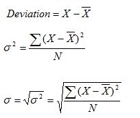
However, when the data of a sample are used to estimate the variance of the population from which the sample was drawn, the population variance estimate is computed instead:
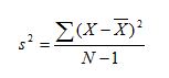
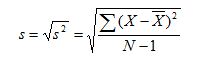
Summary of the calculation procedures:
- subtract the mean from each score
- square each result
- sum all the square
- divide the sum of square by N. Now you get variance
If divide the sum of square by N-1, you will get the population variance estimate
- Standard deviation is just the positive square root of the variance
P13: Prepare and operating statement reconciling budgeted and actual results:
Period: most recent $
Budgeted Profit (50,000 units × $8 per unit profit) 400,000
Sales volume profit variance 80,000 adverse
Standard profit from actual sales (40,000 units × $8 per unit profit) 320,000
Variances (F) (A)
$ $
Sales price 10,000
Direct material price (6,000)
Direct material usage 2,000
Direct labour rate (8,000)
Direct labour efficiency (3,000)
Variable overhead expenditure 6,000
Variable overhead efficiency (4,000)
Fixed overhead expenditure 12,000
Fixed overhead volume (28,000) (7,000)
30,000 (28,000) 2,000
Actual profit 322,000
FIGURE 2: cost reconciliation statement – standard absorption costing
Period: most recent $
Budgeted cost (50,000 units × $12 per unit standard cost) 600,000
Cost volume variance (10,000 units × $12 per unit standard cost) 120,000 favourable
Standard cost of actual production (40,000 units × $12 per unit standard cost) 480,000
Variances (F) (A)
$ $
Direct material price (6,000)
Direct material usage 2,000
Direct labour rate (8,000)
Direct labour efficiency (3,000)
Variable overhead expenditure 6,000
Variable overhead efficiency (4,000)
Fixed overhead expenditure 12,000
Fixed overhead volume (7,000 (7,000) (7,000)
20,000 (28,000) (8,000)
Actual total cost 488,000
Period: most recent
Budgeted contribution (50,000 units × $8.70) 435,000
Sales volume contribution variance (87,000) adverse
Standard contribution from actual sales (40,000 × $8.70) 348,000
Variances (F) (A)
$ $
Sales price 10,000
Direct material price (6,000)
Direct material usage 2,000
Direct labour rate (8,000)
Direct labour efficiency (3,000)
Variable overhead expenditure 6,000
Variable overhead efficiency (7,000 (4,000)
18,000 (21,000) (3,000)
Actual contribution 345,000
Fixed costs $
Budget 35,000
Expenditure variance (12,000) favourable
Actual fixed overhead 23,000
Actual profit 322,000
Period: most recent $
Budgeted variable cost (50,000 units × $11.30 per unit standard cost) 565,000
Cost volume variance (10,000 units × $11.30 per unit standard variable cost) 113,000 favourable
Standard variable cost of actual production 452,000
(40,000 units × $11.30 per unit standard variable cost)
Variances (F) (A)
$ $
Direct material price (6,000)
Direct material usage 2,000
Direct labour rate (8,000)
Direct labour efficiency (3,000)
Variable overhead expenditure 6,000
Variable overhead efficiency 4,000 (4,000)
8,000 (21,000) (13,000)
Actual variable cost 465,000
Fixed costs $
Budget 35,000
Expenditure variance (12,000) favourable
Actual fixed overhead 23,000
Actual total cost 488,000
P14: Report findings to management in accordance with identified responsibility centres:
The use of the responsibility centres concept to structure an organization
In principle the Board of Management has the authority to make decisions within a multinational
enterprise (MNE). Decisions by the highest management level within an enterprise about delegation of
this authority or decentralization will be influenced by the following four factors:
Maximum span of control
The management style concerning the control and steering of the MNE
Transaction costs
The strategy and the business model applied by the MNE.
By delegation of its authority the top management will determine how a manager to whom authority is
delegated will be compensated and/or how the manager will be steered and controlled.
Example: The Management Board of a French MNE gives the sales director of its German sales company
the task to double turnover within a period of 3 years. In this case, one can opt to give the sales director a
bonus on the basis of (a) solely the doubling of turnover or (b) a minimum required level of profitability
of the sales company. The choice between a revenue centre (situation (a)) and a profit centre (situation
(b)) depends on the four factors above. Also, in making this choice it is important to what degree the
German sales company is considered to be able to manage and control the functions and risks related to
situation (b). This information can generally be obtained on the basis of the traditional functional analysis
techniques as described in the OECD Transfer Pricing Guidelines.
In summary, no cases are the same in practice in respect of the choices of roles and responsibilities.
However, in order to structure the analysis of an existing situation, a number of tools are given below,
describing the features of the most common types of responsibility centres.
The following descriptions address the following variables:
The relationship between inputs and outputs of the responsibility centre determines the label. A
responsibility centre can in practice consist of a department, a business unit, a legal entity, a
geographical unit etc.
A description of the type of activities which are common per responsibility centre
A number of examples per responsibility centre
The steering and control concept per responsibility centre
The most common compensation method, both from a management and a tax perspective
The legal framework.
Practical descriptions of responsibility centres
The following schedules are illustrations of the classification of certain activities as an expense centre,
cost centre, revenue centre, profit centre or investment centre. In addition to the usual analysis of
functions, risks and the use of assets per part of the MNE, the responsibility centre label adds a more
process-oriented view on to the MNE, whereby one tries to identify (a) roles and responsibilities within a
MNE and (b) value-added decisions.
Example: In the Italian parent company of a MNE all business decisions are made, whereas the parent
company through the compensation method applied has been classified as a cost centre. The costs of the
parent company are charged to the Belgian subsidiary, which formally acts a principal company – in other
words, it gets the classification “profit centre”. However, taking into account that the staffing in Belgium
is limited to factory workers, the responsibility centre labels – given the allocation of roles between Italy
and Belgium – appear to be in conflict with the economic reality in terms of value-adding decision
making.
Expense centres
Relationship ‘input’/’output’
– inputs are expressed in euros, outputs in units
– output level and cost standards not or hard to determine
Type of activities
– strategically or operationally necessary
– (almost) exclusively performed for group
– mostly core
Examples
– highly creative, non repetitive tasks, e.g. core research
– corporate strategy department, e.g. strategic marketing
Towards steering/control
– determine expense/cost level (= budget)
– monitor actual expenses/cost per department / account
– focus on quality of processes, people and technology applied
Common transfer pricing policy
– actual cost are charged or allocated to recipient (budgeted costs +/- variances)
– actual cost/benefit ratio is frequently reviewed
– profit margin is meaningless from a managerial point of view
– profit margin will be required for tax purposes
Legal framework
– mostly development contract or service level agreement
Cost centres (= engineered expense centres)
Relationship ‘input’/’output’
– inputs are expressed in euros, outputs in units
– output level and cost standards can be determined
Type of activities
– operational activities, managed by principal entity
– mostly performed for group
– mostly non-core
Examples
– subcontracting of manufacturing activities
– facility management activities
– supporting activities of treasury department
– IT system maintenance activities
Towards steering/control
– determine cost standards/targets per product etc.
– monitor actual costs per product etc
– analyse controllable and non-controllable variances
– focus on cost/quality relationship
– allows benchmarking of equivalent activities
Common transfer pricing policy
– standard cost times actual volumes are charged
– sometimes non-controllable variances are settled
– to apply a profit mark-up creates ‘pseudo profit centre’
– profit margin could be applied from a managerial point of view
– profit margin will be required for tax purposes, unless a third party would not be able to charge a
mark-up
Legal framework
– mostly service level agreement
Revenue centres
Relationship ‘input’/’output’
– inputs and outputs are expressed in euros
– output level and cost level not directly related
Type of activities
– market/customer driven activities
– mostly performed for external customers
– mostly core
Examples
– sales and distribution activities
Towards steering/control
– determine and monitor revenue levels
– maximize quantities or prices
Common transfer pricing policy
– allocation of (contribution) margin of sales revenue
Legal framework
– mostly service level agreements (e.g. distribution company)
Profit centres
Relationship ‘input’/’output’
– inputs and outputs are expressed in euros
– output level and cost standards can be determined
Type of activities
– market/customer driven activities
– mostly performed for external customers
– mostly core
Examples
– distribution activities
– speculative activities of treasury department
Towards steering/control
– determine price levels and cost standards per product
– monitor turnover, costs and profits per product
– analyse variances
– focus on profit contribution and quality
Common transfer pricing policy
– external/market price times actual volumes are charged
– operating profit margin should – as primary way of measuring profitability – provide an
adequate return on capital employed for
Legal framework
– mostly service level agreement with ‘cost centres’
Investment centres
Relationship ‘input’/’output’
– inputs and outputs are expressed in euros
– relates profits to assets/underlying capital (=input)
Type of activities
– capital market/customer driven activities
– mostly performed for shareholders/MNO as a whole
– core
Examples
– intellectual property owners (return on investment on R&D)
Towards steering/control
– determine minimum required return on investment
– monitor capital employed and profits per product
– analyse variances on return on investments
– focus on sustaining long term profitability of MNO
Common transfer pricing policy1
– EVA or RONA/ROCE measures should allow monitoring an adequate return on investment
– remuneration based on residual income
Legal framework
– wide variety of legal agreements (if any)