Executive Summery
In this project, Digital Communication System using QPSK Modulation is analyzed and simulated. The main aim of the thesis is to achieve the best digital communication using QPSK modulation and reduce the effect of noises in the communication channel. This thesis details the software implementation of a modern digital communication system and digital modulation methods. The digital modulation schemes considered here include both baseband and Quadrature Phase Shift Keying (QPSK) techniques. The proposed communication system will serve as a practical tool useful for simulating the transmission of any digital data. We use the MATLAB programming to simulate the communication project and simulated portion are attached and discuss briefly. There are some steps of any digital communication model. We discuss each of the steps using necessary diagram and try to understand the reader nicely about digital communication system where we told about Linear Predictive Coding (LPC) in source coding, PLL and all the modulation technique specially the Quadrature Phase Shift Keying (QPSK) in detail for using in the digital communication. The proposed communication system will serve as a practical tool useful for simulating the transmission of any digital data. The various modules of the system include analog to digital converters, digital to analog converters, encoders/decoders and modulators/demodulators. The results show the viability of a QPSK modulated digital communications link.
INTRODUCTION
Communication has been one of the deepest needs of the human race throughout recorded history. It is essential to forming social unions, to educating the young, and to expressing a myriad of emotions and needs. Good communication is central to a civilized society.
The various communication disciplines in engineering have the purpose of providing technological aids to human communication. One could view the smoke signals and drum rolls of primitive societies as being technological aids to communication, but communication technology as we view it today became important with telegraphy, then telephony, then video, then computer communication, and today the amazing mixture of all of these in inexpensive, small portable devices.
Initially these technologies were developed as separate networks and were viewed as having little in common. As these networks grew, however, the fact that all parts of a given network had to work together, coupled with the fact that different components were developed at different times using different design methodologies, caused an increased focus on the underlying principles and architectural understanding required for continued system evolution.
The possible configurations of the link are numerous, so focus was maintained on a typical system that might be used in satellite communications. For this reason convolution channel coders and QPSK modulation were chosen. Additionally, channel effects were primarily modeled as the combination of band laired additive white Gaussian noise (AWGN) and signal attenuation. The results of this link on speech transmission show the various gains and tradeoffs that are realized as data passes through the entire system; the quantitative performance is measured by the probability of bit error, Pe, and the effect various signal to noise ratios have on this probability.
The idea of converting an analog source output to a binary sequence was quite revolutionary in 1948, and the notion that this should be done before channel processing was even more revolutionary. By today, with digital cameras, digital video, digital voice, etc., the idea of digitizing any kind of source is commonplace even among the most technophobic. The notion of a binary interface before channel transmission is almost as commonplace. For example, we all refer to the speed of our internet connection in bits per second.
There are a number of reasons why communication systems now usually contain a binary interface between source and channel (i.e., why digital communication systems are now standard). These will be explained with the necessary qualifications later, but briefly they are as follows:
– Digital hardware has become so cheap, reliable, and miniaturized, that digital interfaces are eminently practical.
– A standardized binary interface between source and channel simplifies implementation and understanding, since source coding/decoding can be done independently of the channel, and, similarly, channel coding/decoding can be done independently of the source.
This thesis studies the Digital Communication System for Quadrature Phase Shift Keying (QPSK) modulation used in digital communications. Software implementation is performed in the MATLAB programming languages and consists of separately coding and interfacing the various functions of the system. By modularizing the various functions which are performed on the data from source to destination, it becomes convenient to change individual sections of the link and model the effects of different transmission conditions on data as it is passed through the channel. The modules of the link include source encoders/decoders, channel encoders/decoders, modulators/demodulators, and channel effects.
ORGANIZATION OF THE THESIS
We use Quadrature Phase Shift Keying (QPSK) Technique in the Digital communication system for better signal transmit and receive in the communication model.
In chapter one, the use and necessary of digital communication in our life has been presented in brief.
In chapter two, we describe the basic digital communication system and channel model which is use in this thesis.
In chapter three, source coding is described briefly. The source encoder is responsible for producing the digital information which will be manipulated by the remainder of the system.
In chapter four, we describe the channel coding in brief and the goal of channel coding is told which allows the detector at the receiver to detect and/or correct errors which might have been introduced during transmission. We use AWGN in the channel coding and it is also presented.
In chapter five, we describe the modulation technique of the digital communication in which Quadrature Phase Shift Keying (QPSK) is described elaborately.
In chapter six, the channel equalization and adaptive filtering are presented in brief.
In chapter seven, we described the demodulation of the communication model used in the thesis.
In chapter eight, we demonstrate the simulation result of QPSK modulation. The software for the simulation, we use the MATLAB platform.
A conclusion was made in chapter nine.
Literature Review
Chapter 2
DIGITAL COMMUNITION MODEL
In this chapter, we describe the basic digital communication system and channel model which is use in this thesis. The model is a simple model of digital communication system. The model is broken into its constituent functions or modules, and each of these is in turn described in terms of its affects on the data and the system. Since this model comprises the entire system, both the source coding and channel equalization are briefly described. In chapters 3 through 8, these two areas will be covered in detail, and the specific algorithms and methods used in the software implementation will be addressed in detail.
We organize this chapter as follows. First, we review some basic notions from digital communications. We present one basic model of digital communication system. We then talk about source encoding and decoding, channel encoding and decoding, modulation, digital interface and channel effects.
2.1 DIGITAL COMMUNICATION
Communication systems that first convert the source output into a binary sequence and then convert that binary sequence into a form suitable for transmission over particular physical media such as cable, twisted wire pair, optical fiber, or electromagnetic radiation through space.
Digital communication systems, by definition,are communication systems that use such a digital sequence as an interface between the source and the channel input (and similarly between the channel output and final destination).
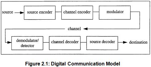
Figure 2.1 in the basic digital communication model the first three blocks of the diagram (source encoder, channel encoder, and modulator) together comprise the transmitter .The source represents the message to be transmitted which includes speech, video, image, or text data among others. If the information has been acquired in analog form, it must be converted into digitized form to make our communication easier. This analog to digital conversion (ADC) is accomplished in the source encoder block. Placing a binary interface between source and channel. The source encoder converts the source output to a binary sequence and the channel encoder (often called a modulator) processes the binary sequence for transmission over the channel.
The last three blocks consisting of detector/demodulator, channel decoder, and source decoder form the receiver. The destination represents the client waiting for the information. This might include a human or a storage device or another processing station. In any case, the source decoder’s responsibility is to recover the information from the channel decoder and to transform it into a form suitable for the destination. This transformation includes digital to analog conversion (DAC) if the destination is a human waiting to hem or view the information or if it is an analog storage device. If the destination is a digital storage device, the information will be kept in its digital state without DAC. The channel decoder (demodulator) recreates the incoming binary sequence (hopefully reliably), and the source decoder recreates the source output.
2.2 SOURCE ENCODING AND ECODING
The source encoder and decoder in Figure 2.1 have the function of converting the input from its original form into a sequence of bits. As discussed before, the major reasons for this almost universal conversion to a bit sequence are as follows: inexpensive digital hardware, standardized interfaces, layering, and the source/channel separation theorem.
The simplest source coding techniques apply to discrete sources and simply involve representing each successive source symbol by a sequence of binary digits. For example, letters from the 27symbol English alphabet (including a space symbol) may be encoded into 5-bit blocks. Since there are 32 distinct 5-bit blocks, each letter may be mapped into a distinct 5-bit block with a few blocks left over for control or other symbols. Similarly, upper-case letters, lower-case letters, and a great many special symbols may be converted into 8-bit blocks (“bytes”) using the standard ASCII code.
For example the input symbols might first be segmented into m – tupelos, which are then mapped into blocks of binary digits. More generally yet, the blocks of binary digits can be generalized into variable-length sequences of binary digits. We shall find that any given discrete source, characterized by its alphabet and probabilistic description, has a quantity called entropy associated with it. Shannon showed that this source entropy is equal to the minimum number of binary digits per source symbol required to map the source output into binary digits in such a way that the source symbols may be retrieved from the encoded sequence.
Some discrete sources generate finite segments of symbols, such as email messages, that are statistically unrelated to other finite segments that might be generated at other times. Other discrete sources, such as the output from a digital sensor, generate a virtually unending sequence of symbols with a given statistical characterization. The simpler models of Chapter 2 will correspond to the latter type of source, but the discussion of universal source coding is sufficiently general to cover both types of sources, and virtually any other kind of source.
The most straight forward approach to analog source coding is called analog to digital (A/D) conversion.
2.3 CHANNEL ENCODING AND DECODING
The channel encoder and decoder box in Figure 2.1 has the function of mapping the binary sequence at the source/channel interface into a channel waveform.
One of the advantages of digital communications over analog communications is its robustness during transmission. Due to the two state nature of binary data (i.e. either a 1 or a 0), it is not as susceptible to noise or distortion as analog data. While even the slightest noise will corrupt an analog signal, small mounts of noise will generally not be enough to change the state of a digital signal from I to 0 or vice versa and will in fact be ‘ignored’ at the receiver while the correct information is accurately recovered.
Nevertheless, larger amounts of noise and interference can cause a signal to be demodulated incorrectly resulting in a bit stream with errors at the destination. Unlike an analog system, a digital system can reduce the effect of noise by employing an error control mechanism which is used prior to modulation. The channel encoder performs this error control by systematically introducing redundancy into the information bit stream after it has been source encoded but prior to its transmission. This redundancy can then be used by the receiver to resolve errors that might occur during transmission due to noise or interference.
The channel decoder performs the task of decoding the received coded bit stream by means of a decoding algorithm tailored for the encoding scheme. Error control of this variety that allows a receiver to resolve errors in a bit stream by decoding redundant information introduced at the transmitter is known as Forward Error Correction (FEC). The price paid for employing FEC is the increased bit rate and complexity of the transmitter and receiver.
2.4 MODULATION
The digital modulator serves as an interface between the transmitter and the channel. It serves the purpose of mapping the binary digital information it receives into waveforms compatible with the channel. In baseband modulation, the output waveforms we simple voltage pulses which take predefined values corresponding to a 1 or 0. However, many channels, such as a satellite channel, are not suited for backhand communication and require the incoming data to be modulated to a higher frequency, referred to as the carrier frequency, so it can be converted to an electromagnetic wave that will propagate through space to its destination ( a satellite or a ,round station) This type of modulation, known as band pass modulation, varies one of the following three parameters of the carrier frequency based on the incoming digital bit stream: amplitude, frequency or phase. These modulation types are commonly known as Amplitude Shift Keying (ASK). Frequency Shift Keying (FSK) and Phase Shift Keying (PSK) respectively.
The digital detector/demodulator reverses the process and extracts the binary baseband information from the received modulated signal which has been subjected to noise, interference, loss, and other distortions. The demodulator produces a sequence of binary values which are estimates of the transmitted data and passes it on to the channel decoder.
2.5 DIGITAL INTERFACE
The interface between the source coding layer and the channel coding layer is a sequence of bits. However, this simple characterization does not tell the whole story. The major complicating factors are as follows:
– Unequal rates: The rate at which bits leave the source encoder is often not perfectly matched to the rate at which bits enter the channel encoder.
– Errors: Source decoders are usually designed to decode an exact replica of the encoded sequence, but the channel decoder makes occasional errors.
– Networks: Encoded source outputs are often sent over networks, traveling serially over several channels; each channel in the network typically also carries the output from a number of different source encoders.
The first two factors above appear both in point-to-point communication systems and in networks. They are often treated in an ad hoc way in point-to-point systems, whereas they must be treated in a standardized way in networks. The third factor, of course, must also be treated in a standardized way in networks.
2.6 CHANNEL EFFECTS
During transmission, the signal undergoes various degrading and distortion effects as it passes through the medium from the transmitter to the receiver. This medium is commonly referred to as the channel. Channel effects include, but are not limited to, noise, interference, linear and non linear distortion and attenuation. These effects are contributed by a wide variety of sources including solar radiation, weather and signals front adjacent channels. But many of the prominent effects originate from the components in the receiver. While many of the effects can be greatly reduced by good system design, careful choice of filter parameters, and coordination of frequency spectrum usage with other users, noise and attenuation generally cannot be avoided and are the largest contributors to signal distortion.
In digital communication systems, a common quantity used to determinate whether a signal will be detected correctly is the ratio of energy per bit to spectral noise power density, Eb / No, measured at the detector. The higher the Eb, the lower the resulting bit error rate (BER), the probability of bit error, Pb Unfortunately, a high Eb demands greater power consumption at the transmitter; in some cases, it may be unfeasible to obtain a high Eb due to transmitter size or power limitations as in the case of satellite transmission.
The digital communication system described consists of an ordered grouping of various modules which operate on an input data sequence. In practice, these modules or resources are not dedicated to a single source/destination, but they me shared by multiple sources and their destinations to achieve optimum utilization.
In a digital system, the transmission bit rate is an important system resource. A given information source of bandwidth B, sampled at 2B samples/second using q bits per sample results in a data rate, R, of 2Bq bits per second. With a compression ratio C, the data rate from the source encoder is Rs = RIC bits per second. Channel coding by a factor n leads to a coded data rate of Rc = Rs n bits per second; R, is the system transmission bit rate. These bits we then used by the modulator to form the transmission waveforms which have to be accommodated within the available bandwidth. At the receiver these steps m performed in the reverse order to recover the information sequence.
Chapter 3
SOURCE CODING
In the digital communication system model described previously, the source encoder is responsible for producing the digital information which will be manipulated by the remainder of the system. After the digital signal is acquired from the analog information, the source encoder subjects it to a wide range of processing functions, the goals of which are to compactly represent the information. Speech, image, and textual information each have their own unique characteristics that require different source encoding techniques. Depending on the information source, different digital signal processing functions are implemented to remove the redundancies inherent in the given signal. The specifics of the speech compression techniques used in this thesis are detailed below.
In this chapter we describe the source coding and then its related speech compression, Linear predictive coding (LPC) and Code excited linear prediction (CELP).The use of these in digital communication in source coding. And we also describe the LPC in large as we use it in the source coding in our digital communication thesis.
3.1 SPEECH COMPRESSION
Since the frequency content of spoken language is confined to frequencies under 4000 Hz, it is reasonable to use a sampling frequency of 8000 Hz. Using 16 bit linear Pulse code modulation (PCM) as the quantization method results in a bit rate of 128 kbps. Subsequent analysis, coding, and compression of speech are performed on segments or frames of 20 to 30 ms duration.
There are two broad categories of speech coding/compression. Both categories are concerned with representing the speech with the minimum number of applicable parameters while also allowing the speech to be intelligibly reproduced; both are loss in nature.
The first category deals with waveform coders which manipulate quantities in the speech signal’s frequency representation. Typical analysis tools of waveform coders are the Discrete Fourier Transform (DFT) and the Discrete Wavelet Transform (DWT), both of which transform the time signal to its frequency domain representation. In this case, compression might potentially be achieved by retaining the frequency components with the largest magnitudes.
The second category of speech compression deals with voice coders, or vocoders for short. Vocoders attempt to represent speech as the output of a linear system driven by either periodic or random excitation sequences as shown in Figure 3.1.
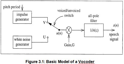
A periodic impulse train or a white noise sequence, representing voiced or unvoiced speech, drives an all pole digital filter to produce the speech output. The all pole filter digital filter models the vocal tract.
Additionally, estimates of the pitch period and gain parameters are necessary for accurate reproduction of the speech. Due to the slowly changing shape of the vocal tract over time, vocoders successfully reproduce speech by modeling the vocal tract independently for each frame of speech and driving it by an estimate of a separate input excitation sequence for that frame. Most vocoders differ in performance principally based on their methods of estimating the excitation sequences.
3.2 LINEAR PREDICTIVE CODING (LPC)
Linear Predictive Coding (LPC) is one of the most powerful speech analysis techniques, and one of the most useful methods for encoding good quality speech at a low bit rate. It provides extremely accurate estimates of speech parameters, and is relatively efficient for computation. This document describes the basic ideas behind linear prediction, and discusses some of the issues involved in its use.
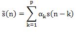
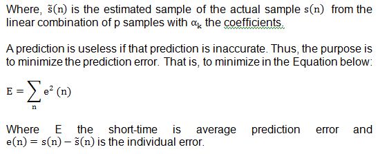
Linear prediction model speech waveforms are same by estimating the current value from the previous values. The predicted value is a linear combination of previous values. The linear predictor coefficients are determined such that the coefficients minimize the error between the actual and estimated signal. The basic equation of linear prediction is given as follows:
LPC starts with the assumption that the speech signal is produced by a buzzer at the end of a tube. The glottis (the space between the vocal cords) produces the buzz, which is characterized by its intensity (loudness) and frequency (pitch). The vocal tract (the throat and mouth) forms the tube, which is characterized by its resonances, which are called formants. For more information about speech production, see the Speech Production OLT.
LPC analyzes the speech signal by estimating the formants, removing their effects from the speech signal, and estimating the intensity and frequency of the remaining buzz. The process of removing the formants is called inverse filtering, and the remaining signal is called the residue.
The numbers which describe the formants and the residue can be stored or transmitted somewhere else. LPC synthesizes the speech signal by reversing the process: use the residue to create a source signal, use the formants to create a filter (which represents the tube), and run the source through the filter, resulting in speech.
Because speech signals vary with time, this process is done on short chunks of the speech signal, which are called frames. Usually 30 to 50 frames per second give intelligible speech with good compression.
A. Speech Production
When a person speaks, his or her lungs work like a power supply of the speech production system. The glottis supplies the input with the certain pitch frequency (F0). The vocal tract, which consists of the pharynx and the mouth and nose cavities, works like a musical instrument to produce a sound. In fact, different vocal tract shape would generate a different sound. To form different vocal tract shape, the mouth cavity plays the major role. To produce nasal sounds, nasal cavity is often included in the vocal tract. The nasal cavity is connected in parallel with the mouth cavity. The simplified vocal tract is shown in Fig 3.2.
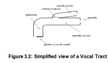
The glottal pulse generated by the glottis is used to produce vowels or voiced sounds. And the noise-like signal is used to produce consonants. ..or unvoiced sounds.
B. Linear Prediction Model
An efficient algorithm known as the Levinson-Durbin algorithm is used to estimate the linear prediction coefficients from a given speech waveform.
Assume that the present sample of the speech is predicted by the past M samples of the speech such that
Where the prediction of is is the kth step previous sample, and ak are called the linear prediction coefficients.
The transfer function is given by
Because ε(n), residual error, has less standard deviation and less correlated than speech itself, smaller number of bits is needed to quantize the residual error sequence. Equation can be rewritten as the difference equation of a digital filter whose input is ε (n) and output is s (n) such that
The implementation of the above equation is called the synthesis filter and is shown in Figure 3.5.
If both the linear prediction coefficients and the residual error sequence are available, the speech signal can be reconstructed using the synthesis filter. In practical speech coders, linear prediction coefficients and residual error samples need to be compressed before transmission. Instead of quantizing the residual error, sample by sample, several important parameters such as pitch period, code for a particular excitation, etc are transmitted. At the receiver, the residual error is reconstructed from the parameters.
3.3 CODE EXCITED LINEAR PEDICTION (CELP)
Although the data rate of plain LPC coders is low, the speech reproduction, while generally intelligible, has a metallic quality, and the vocoder artifacts are readily apparent in the unnatural characteristics of the sound. The reason for this is because this algorithm does not attempt to encode the excitation of the source with a high degree of accuracy. The CELP algorithm attempts to resolve this issue while still maintaining a low data rate.
Speech frames in CELP are 30 ms in duration, corresponding to 240 samples per frame using a sampling frequency of 8000 Hz. They are further partitioned into four 7.5 ms sub frames of 60 samples each. The bulk of the speech analysis/synthesis is performed over each sub frame.
The CELP algorithm uses two indexed codebooks and three lookup tables to access excitation sequences, gain parameters, and filter parameters. The two excitation sequences are scaled add summed to form the input excitation to a digital filter created from the LPC filter parameters. The codebooks consist of sequences which are each 60 samples long, corresponding to the length of a sub frame.
CELP is referred to as an analysis by synthcsis technique.
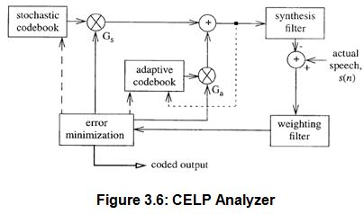
Figure 3.6 shows a schematic diagram of the CELP analyzer/coder. The stochastic codebook is fixed containing 512 zero mean Gaussian sequences. The adaptive codebook has 256 sequences formed from the input sequences to the digital filter and updated every two sub frames. A code from the stochastic codebook is scaled and summed with a gain scaled code from the adaptive codebook.
The result is used as the input excitation sequence to an LPC synthesis filter. The output of the filter is compared to the actual speech signal, and the weighted error between the two is compared to the weighted errors produced by using all of the other codewords in the two codebooks. The codebook indices of the two codewords (one each from the stochastic add adaptive codebooks), along with their respective gains, which minimize the error are then coded for transmission along with the synthesis filter (LPC) parameters. Because, the coder passes each of the adaptive and stochastic codewords through the synthesis filter before selecting the optimal codewords.
Chapter 4
CHANNEL CODING
We considered the problem of digital modulation by means of M=2k signal waveforms, where each waveform conveys k bits of information. We observed that some modulation methods provide better performance than others. In particular, we demonstrated that orthogonal signaling waveforms allow us to make the probability of error arbitrarily mail by letting the number of waveforms M → ∞ provided that the SNR per bit γb ≥ 1.6 dB. Thus, we can operate at the capacity of the Additive White Gaussian Noise channel in the limit as the bandwidth expansion factor Be =W/R→∞. This is a heavy price to pay, because Be grows exponentially with the block length k. Such inefficient use of channel bandwidth is highly undesirable.
In this and the following chapter, we consider signal waveforms generated from either binary or no binary sequences. The resulting waveforms are generally characterized by a bandwidth expansion factor that grows only linearly with k. Consequently, coded waveforms offer the potential for greater bandwidth efficiency than orthogonal M ary waveforms. We shall observe that. In general, coded waveforms offer performance advantages not only in power limited applications where RIW<1, but also in bandwidth limited systems where R/W > 1.
We begin by establishing several channel models that will be used to evaluate the benefits of channel coding, and we shall introduce the concept of channel capacity for the various channel models, then, we treat the subject of code design for efficient communications.
4.1 CHANNEL MODEL
In the model of a digital communication system described in chapter 2, we recall that the transmitter building block; consist of the discrete input, discrete output channel encoder followed by the modulator. The function of the discrete channel encoder is to introduce, in a controlled manner, some redundancy in the binary information sequence, which can be used at the receiver to overcome the effects of noise and interference encountered in the transmission of the signal through the channel. The encoding process generally involves taking k information bits at a time and mapping each k bit sequence into a unique n bit sequence, called a code word. The amount of redundancy introduced by the encoding of the data in this manner is measured by the ratio n/k. The reciprocal of this ratio, namely k/n, is called the code rate.
The binary sequence at the output of the channel encoder is fed to the modulator, which serves as the interface to the communication channel. As we have discussed, the modulator may simply map each binary digit into one of two possible waveforms, i.e., a 0 is mapped into s1 (t) and a 1 is mapped into S2 (t). Alternatively, the modulator may transmit q bit blacks at a time by using M = 2q possible waveforms.
At the receiving end of the digital communication system, the demodulator processes the channel crurrupted waveform and reduces each waveform to a scalar or a vector that represents an estimate of the transmitted data symbol (binary or M ary).The detector, which follows the demodulator, may decide on whether the ‘transmitted bit is a 0 or a 1. In such a case, the detector has made a hard decision. If we view the decision process at the detector as a form of quantization, we observe that a hard decision corresponds to binary quantization of the demodulator output. More generally, we may consider a detector that quantizes to Q > 2 levels, i.e. a Q ary detector. If M ary signals are used then Q ≥ M. In the extreme case when no quantization is performed, Q = M. In the case where Q > M, we say that the detector has made a soft decision.
A. Binary Symmetric Channel
Figure 4.1: A composite discrete-input, discrete output channel
Let us consider an additive noise channel and let the modulator and the demodulator/detector be included as parts of the channel. If the modulator employs binary waveforms and the detector makes hard decisions, then the composite channel, shown in Fig. 4.1, has a discrete-time binary input sequence and a discrete-time binary output sequence. Such a composite channel is characterized by the set X = {0, 1} of possible inputs, the set of Y= {0, 1} of possible outputs, and a set of conditional probabilities that relate the possible outputs to the possible inputs. If the channel noise and other disturbances mum statistically independent errors in the transmitted binary sequence with average probability P then,
P(Y = 0 / x = 1) = P(Y = 1 / x = 0) = P
P(Y = 1 / x = 1) = P(Y = 0 / X = 0) = 1- P
Thus, we have reduced the cascade of the binary modulator, the waveform channel, and the binary demodulator and detector into an equivalent discrete-time channel which is represented by the diagram shown in Fig 4.1. This binary-input, binary-output, symmetric channel is simply called a binary symmetric channel (BSC).
B. Discrete Memory Less Channel
The BSC is a special can of a more general discrete-input, discrete-output channel. Suppose that the output form the channel encoder are q ary symbols, i.e., X={x0, x1,…,xq -1) and the output of the decoder consists of q ary symbols, where Q ≥M =2q.
Figure 4.2: Binary symmetric channels
If the channel and the modulation are memory less, then the input-output characteristics of the composite channel, shown in Fig. 4.1, are described by a set of qQ conditional probabilities.
C. Waveform Channels
We may separate the modulator and demodulator from the physical channel, and consider a channel model in which the inputs are waveforms and the outputs are waveforms. Let us assume that such a channel has a given bandwidth W, with ideal frequency response C(f) =1 within the bandwidth W, and the signal at its output is corrupted by additive white Gaussian noise. Suppose that x (t) is a band-limited input to such a channel and y (t) is the corresponding output, then,
y(t) = x(t) + n(t)
Where n(t) represents a sample function of the additive noise process.
4.2 CONVOLUTIONAL CODES
For (n,1) convolution codes, each bit of the information sequence into the encoder results in an output of n bits. However, unlike block codes, the relationship between information bits and output bits is not a simple one-to-one mapping. In fact, each input information bit is ‘convolved’ with K-1 other information bits to form the output n bit sequence. The value K is known as the constraint length of the code and is directly related to its encoding and decoding complexity as described below in a brief explanation of the encoding process.
For each time step, an incoming bit is stored in a K stage shift register, and bits at predetermined locations in the register are passed to n modulo 2 adders to yield the n output bits. Each input bit enters the first stage of the register, and the K bits already in the register are each shifted over one stage with the last bit being discarded from the last stage.
The n output bits produced by the entry of each input bit have a dependency on the preceding K-1 bits. Similarly, since it is involved in the encoding of K-1 input bits in addition to itself, each input bit is encoded in nK output bits. It is in this relationship that convolutional coding derives its power. For larger values of K, the dependencies among the bits increased the ability to correct more errors rises correspondingly. But the complexity of the encoder and especially of the decoder also becomes greater.
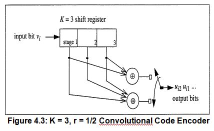
Shown in Figure 4.3 is the schematic for a (2,1) encoder with constraint length K= 3 which will serve as the model for the remainder of the development of convolutional coding. In the coder shown, the n = 2 output bits are formed by modulo 2 addition of the bits in stages one and three and the addition of bits in stages one, two, and three of the shift register.
Chapter 5
MODULATION
In this chapter, we describe the basic Modulation Technique and emphasis on QPSK Modulation which is use in this thesis. We are trying to show how QPSK Modulation is used in digital communication system. In digital transmission systems, the data sequence from the channel encoder is partitioned into L bit words, and each word is mapped to one of M corresponding waveforms according to some predetermined rule, where M = 2L. We shall see later, in a QPSK modulation system, the incoming sequence is separated into words of L = 2 bits each and mapped to M = 22 = 4 different waveforms. During transmission, the channel causes attenuation and introduces noise to the signal. The net result is the formation of a version of the original signal which may not be detected correctly by the receiver. If the errors are too numerous, the channel decoder may not be able to resolve the information correctly. Baseband modulation using the simple binary symmetric channel model is briefly discussed, and the details of QPSK modulation are then presented.
We organize this chapter as follows. First, we review some basic from Modulation Technique. We present basic modulation of Amplitude Shift-keying (ASK), Frequency Shift-keying(FSK),Phase Shift-keying(PSK), Binary Phase Shift-keying (BPSK) and Quadrature Phase Shift-keying(QPSK). We then talk about Quadrature Phase Shift-keying(QPSK) in detail and try to show the use of QPSK in digital communication system.
5.1 AMPLITUDE SHIFT KEYING (ASK)
In many situations, for example in radio frequency transmission, data cannot be transmitted directly, but must be used to modulate a higher frequency sinewave carrier. The simplest way of modulating a carrier with a data stream is to change the amplitude of the carrier every time the data changes. This technique is known as amplitude shift -keying.
The simplest form of amplitude shift-keying is on- off keying, where the transmitter outputs the sinewave carrier whenever the data bit is a ‘1’, and totally suppresses the carrier when the data bit is ‘0’. In other words, the carrier is turned ‘on’ for a ‘1’, and ‘off ‘ for a ‘0’.This form of amplitude shift-keying is illustrated in figure below:
Figure 5.1: an ASK signal (below) and the message (above)
In order to generate an amplitude shift-keyed (ASK) wave form at the Transmitter a balanced modulator circuit is used (also known as a linear multiplier). This device simply multiplies together the signals at its two inputs, the output voltage at any instant in time being the product of the two input voltages. One of the inputs is a.c. coupled; this is known as the carrier input. The other is d.c. coupled and is known as the modulation (or signal) input.
In order to generate the ASK waveform, all that is necessary is to connect the sine wave carrier to the carrier input, and the digital data stream to the modulation input, as shown in figure below:
Figure 5.2: ASK generation method
The data stream applied to the modulator’s modulation input is unipolar, i.e. its ‘0’ and ‘1’ levels are 0 volts and +5volts respectively. Consequently.
(1) When the current data bit is a ‘1’ , the carrier is multiplied by a constant, positive voltage, causing the carrier to appear, unchanged in phase, at the modulator’s output.
(2) When the current data bit is a ‘0’, the carrier is multiplied by 0 volts, giving 0 volt as at the modulators output.
At the Receiver, the circuitry required to demodulate the amplitude shift- keyed wave form is minimal.The filter’s output appears as a very rounded version of the original data stream, and is still unsuitable for use by the “Receiver’s digital circuits. To overcome this, the filter’s output wave form is squared up by a voltage comparator.
5.2 Frequency Shift-keying
In frequency shift -keying, the signal at the Transmitter’s output is switched from one frequency to another every time there is a change in the level of the modulating data stream For example, if the higher frequency is used to represent a data ‘1’ and the lower ferquency a data ‘0’, the reasulting Frequency shift keyed (FSK) waveform might appear as shown in Figure below:
Figure 5.3 An ASK waveform
The generations of a FSK waveform at the Transmitter can be acheived by generating two ASK waveforms and adding them together with a summing amplifier.
At the Receiver, the frequency shift-keyed signal is decoded by means of a phase-locked loop (PLL) detector. The detector follows changes in frequency in the FSK signal, and generates an output voltage proportional to the signal ferquency.
The phase-locked loop’s output also contains components at the two carrier frequencies; a low-pass fillter is used to filter these components out.
The filter’s output appears as a very rounded version of the original data stream, and is still unsuitable for use by the Receiver’s digital circuits. To overcome this, the filter’s output waveform is squared up by a voltage comparator. Figure below shows the functional blocks required in order to demodulate the FSK waveform at the Receiver.
5.3 Phase Shift keying (PSK)
In phase shift keying the phase of the carrier sinewave at the transmitter’s output is switched between 0 º and 180 º, in sympathy with the data to be transmitted as shown in figure below:
Figure 5.3: phase shift keying
The functional biocks required in order to generate the PSK signal are similar to those required to generate an ASK signal. Again a balanced modulator is used, with a sinewave carrier applied to its carrier input. In contscast to ASK generation, however, the digital signal applied to the madulation input for PSK generation is bipolar, rather than unipolar, that is it has equal positive and negative voltage levels.
When the modulation input is positive, the modulator multiplies the carier input by this constant level. so that the modulator’s output signal is a sinewave which is in phase with the carrier input.
When the modulation input is negative, the modulator multiplies the carrier input by this constant level, so that the modulatior’s autput signal is a sinewave which is 180 º out of phase with the carier input.
At the Receiver, the frequency shift-keyed signal is decoded by means of a squaring loop detector. This PSK Demodulator is shown in figure below:
5.4 BINARY PHASE-SHIFT KEYING (BPSK)
In binary phase shift keying (BPSK), the transmitted signal is a sinusoid of fixed amplitude it has one fixed phase when the data is at one level and when the data is at the other level the phase is different by 180 º . If the sinusoid is of Amplitude A it has a power :
Ps = 1/2 A2
A = Root over (2 Ps)
BPSK(t) = Root over (2 Ps) Cos (ω0t)
BPSK(t) = Root over (2 Ps) Cos (ω0t+π )
= – Root over (2 Ps) Cos (ω0t)
In BPSK the data b(+) is a stream of binary digits with voltage levels which, we take to be at +1V and – 1 V. When b(+) =1V we say it is at logic 1 and when b(+)= -1V we say it is logic 0. Hence, BPSK(t) can be written as:
BPSK(t) = b(t) Root over (2 Ps) Cos (w0t)
In practice a BPSK signal is generated by applying the waveform Coswo as a carrier to a balanced modulator and applying the baseband signal b(+) as the modulating signal. In this sense BPSK can be thought of as an AM signal similar as PSK signal.
5.5 Quadrature Phase Shift Keying (QPSK)
In this section the topics of QPSK modulation of digital signals including their transmission, demodulation, and detection, are developed. The material in this section and the related coding of this system are both based on transmission using an AWGN channel model which is covered at the end of this section. Some of the techniques discussed below are specifically designed for robustness under these conditions.
Because this is a digital implementation of a digital system, it is important to note that the only places where analog quantities occur are after the DAC, prior to the actual transmission of the signal, and before the ADC at the receiver. All signal values between the source encoder input and modulator output are purely digital. This also holds for all quantities between the demodulator and the source decoder.
A. Background
QPSK modulation is a specific example of the more general M ary PSK. For M ary PSK, M different binary words of length L = log2 M bits are assigned to M different waveforms. The waveforms we at the same frequency but separated by multiples of φ = 2π/M in phase from each other and can be represented as follows:
, =
with i = 1, 2, … M. The carrier frequency and sampling frequency are denoted by fc and fs respectively.
Since an M ary PSK system uses L bits to generate a waveform for transmission, its symbol or baud rate is 1IL times its bit rate. For QPSK, there we M = 4 waveforms separated by multiples of ( = ) radians and assigned to four binary words of length L = 2 bits. Because QPSK requires two incoming bits before it can generate a waveform, its symbol or baud rate, D, is one half of its bit rate, R.
B. Transmitter
Figure 5.2 illustrates the method of QPSK generation. The first step in the formation of a QPSK signal is the separation of the incoming binary data sequence, b, into an in phase bit stream, b1, and a quadratic phase bits ream, bQ, as follows. If the incoming data is given by b = bo, b1, b2, b3, b4…. where bi are the individual bits in the sequence, then, bI = bo, b2, b4 ……(even bits of b) and bQ= b1, b3, b5 …… (odd bits). The digital QPSK signal is created by summing a cosine function modulated with the bI, stream and a sine function modulated by the bQ stream. Both sinusoids oscillate at the same digital frequency, ω0=2π fc / fs radians. The QPSK signal is subsequently filtered by a band pass filter, which will be described later, and sent to a DAC before it is finally transmitted by a power amplifier.
Figure 5.4 QPSK Modulator
B.1 Signal Constellation
It is often helpful to represent the modulation technique with its signal space representation in the I Q plane as shown in Figure 5.3. The two axes, I and Q, represent the two orthogonal sinusoidal components, cosine and sine, respectively, which are added together to form the QPSK signal as shown in Figure 5.2. The four points in the plane represent the four possible QPSK waveforms and me separated by multiples of n/2 radians from each other. By each signal point is located the input bit pan which produces the respective waveform. The actual I and Q coordinates of each bit pair are the contributions of the respective sinusoid to the waveform. For example, the input bits (0, 1) in the second quadrant correspond to the (I,Q) coordinates, ( 1,1). This yields the output waveform I + Q = cos (ω0n) + sin (ω0n). Because all of the waveforms of a QPSK have the same amplitude, all four points are equidistant from the origin. Although the two basis sinusoids shown in Figure 5.2 are given by cos (ω0n) and sin (ω0n), the sinusoids can be my two functions that are orthogonal.
Figure 5.3 Signal Constellation of QPSK
B.2 Filtering
The QPSK signal created by the addition of the two sinusoids has significant energy in frequencies above and below the carrier frequency. This is due to the frequency contributions incurred during transitions between symbols which are either 90 degrees or 180 degrees out of phase with each other. It is common to limit the out of band power by using a digital band pass filter (BPF) centered at ωo. The filter has a flat pass band and a bandwidth which is 1.2 to 2 times the symbol rate.
C. Receiver
The receiver’s function consists of two steps: demodulation and detection. Demodulation entails separating the received signal into its constituent components. For a QPSK signal, these are the cosine and sine waveforms carrying the bit information. Detection is the process of determining the sequence of ones and zeros those sinusoids represent.
C.1 Demodulator
The demodulation procedure is illustrated below in Figure 5.4. The first step is to multiply the incoming signal by locally generated sinusoids. Since the incommoding signal is a sum of sinusoids, and the receiver is a linear system, the processing of the signal can be treated individually for both components and summed upon completion.
Figure 5.4: QPSK Demodulator and Detector
Assuming the received signal is of the form
r(n) = AI cos(ω0 n) + AQ sin (ω0 n)
where AI and AQ are scaled versions of the bI and bQ bitstreams used to modulate the signal at the transmitter. The contributions through the upper and lower arms of the demodulator due to the cos(ω0 n) input alone are
rci = AI cos(ω0 n) cos (ω0 n+ ө)
rcQ = AI cos(ω0 n) sin (ω0 n+ ө)
where ө is the phase difference between the incoming signal and locally generated sinuso¬ids. These equations can be expanded using trigonometric identities to yield.
C.2 Detection
After the signal r(n) has been demodulated into the bitstreams dj(n) and dQ(n), the corresponding bit information must be recovered. The commonly used technique is to use a matched filter at the output of each LPF as shown in Figure 5.4. The matched filter is an optimum receiver under AWGN channel conditions and is designed to produce a maximum output when the input signal is a min or image of the impulse response of the filter. The outputs of the two matched filters are the detected bitstreams bdj and bdO, and they are recombined to form the received data bitstream. The development of the matched filter and its statistical properties as an optimum receiver under AWGN conditions can be found in various texts.
5.6 AWGN Channel
The previously introduced BSC channel modeled all of the channel effects with one parameter, namely the BER; however, this model is not very useful when attempting to more accurately model a communication system’s behavior. The biggest drawback is the lack of emphasis given to the noise which significantly corrupts all systems.
The most commonly used channel model to deal with this noise is the additive white Gaussian noise (AWGN) channel model. The time results because the noise is simply added to the signal while the term ‘white’ is used because the frequency content is equal across the entire spectrum. In reality, this type of noise does not exist and is confined to a finite spectrum, but it is sufficiently useful for systems whose bandwidths are small when compared to the noise power spectrum.
Chapter 6
CHANNEL EQUALIZATION
Equalization is partitioned into two broad categories. The first category, maximum likelihood sequence estimation (MLSE), entails making measurements of impulse response and then providing a means for adjusting the receiver to the transmission environment. The goal of such adjustment is to enable the detector to make good estimates from the demodulated distorted pulse sequence. With an MLSE receiver, the distorted samples are not reshaped or directly compensated in any way; instead, the mitigating techniques for MLSE receiver is to adjust itself in such a way that it can better deal with the distorted samples such as Viterbi equalization.
The second category, equalization with filters, uses filters to compensate the distorted pulses. In this second category, the detector is presented with a sequence of demodulated samples that the equalizer has modified or cleaned up from the effects of ISI. The filters can be distorted as to whether they are linear devices that contain only feed forward elements (transversal equalizer), or whether they are nonlinear devices that contain both feed for ward and feedback elements (decision feedback equalizer) the can be grouped according to the automatic nature of their operation, which may either be preset or adaptive.
They are also grouped according to the filter’s resolution or update rate.
Symbol spaced
Pre detection samples provided only on symbol boundaries, that is, one sample per symbol. If so, the condition is known.
Fractionally spaced
Multiple samples provided for each symbol. If so, this condition is known.
6.1 ADAPTIVE EQUALIZATION
An adaptive equalizer is an equalization filter that automatically adapts to time-varying properties of the communication channel. It is frequently used with coherent modulations such as phase shift keying, mitigating the effects of multipath propagation and Doppler spreading. Many adaptation strategies exist. A well-known example is the decision feedback equalizer, a filter that uses feedback of detected symbols in addition to conventional equalization of future symbols. Some systems use predefined training sequences to provide reference points for the adaptation process.
Adaptive equalization is capable of tracking a slow time varying channel response. It can be implemented to perform tap weight adjustments periodically or continually. Periodic adjustments are accomplished by periodically transmitting a preamble or short training sequence of digital data that is known in advance by the receiver. The receiver also detects the preamble to detect start of transmission, to set the automatic gain control level, and to align internal clocks and local oscillator with the received signal. Continual adjustments are accomplished by replacing the known training sequence with a sequence of data symbol estimated from the equalizer output and treated as known data. When performed continually and automatically in this way, the adaptive procedure is referred to as decision directed. Decision directed only addresses how filter tap weights are adjusted-that is with the help of signal from the detector. DFE, however, refers to the fact that there exists an additional filter that operates on the detector output and recursively feed back a signal to detector input. Thus with DFE there are two filters, a feed forward filter and a feed back filter that processes the data and help mitigate the ISI.
Adaptive equalizer particularly decision directed adaptive equalizer, successfully cancels ISI when the initial probability of error exceeds one percent. If probability of error exceeds one percent, the decision directed equalizer might not converge. A common solution to this problem is to initialize the equalizer with an alternate process, such as a preamble to provide good channel error performance, and then switch to the decision directed mode. To avoid the overhead represented by a preamble many systems designed to operate in a continuous broadcast mode use blind equalization algorithms to form initial channel estimates. These algorithms adjust filter coefficients in response to sample statistics rather than in response to sample decisions.
Automatic equalizer use iterative techniques to estimate the optimum coefficients. The simultaneous equations do not include the effects of channel noise. To obtain a stable solution to the filter weights, it is necessary that the data are average to obtain, stable signal statistics or the noisy solution obtained from the noisy data must be averaged considerations of algorithm complexity and numerical stability most often lead to algorithms that average noisy solutions. The most robust of this class of algorithm is the least mean square algorithm.
6.2 LMS ALGORITHM FOR OEFICIENT ADJUSTMENT
Suppose we have an FIR filter with adjustable coefficient {h(k),0<k<N-1}. Let x(n) denote the input sequence to the filter, and let the corresponding output be {y(n)}, where
y(n) = n=0,….M
Suppose we also have a desired sequence d(n) with which we can compare the FIR filter output. Then we can form the error sequence e(n) by taking the difference between d(n) and y(n). That is,
e(n)=d(n)-y(n), n=0,….M
The coefficient of FIR filter will be selected to minimize the sum of squared errors.
Thus we have
+
where, by definition,
rdx(k)= 0 ≤ k ≤ N-1
rxx(k)= 0 ≤ k ≤ N-1
We call rdx(k) the cross correlation between the desired output sequence d(n) and the input sequence x(n), and rxx(k) is the auto correlation sequence of x(n).
The sum of squared errors ε is a quadratic function of the FIR filter coefficient. Consequently, the minimization of ε with respect to filter coefficient h(k) result in a set of linear equations. By differentiating ε with respect to each of the filter coefficients, we obtain,
∂ε /∂h(m)=0, 0 ≤ m ≤ N-1
and, hence
rxx(k-m)=rdx(m), 0 ≤ k ≤ N-1
This is the set of linear equations that yield the optimum filter coefficients.
To solve the set of linear equations directly, we must first compare the autocorrelation sequence rxx(k) of the input signal and cross correlation sequence rdx(k) between the desired sequence d(n) and input sequence x(n).
The LMS provides an alternative computational method for determining the optimum filter coefficients h(k) without explicitly computing the correlation sequences rxx(k) and rdx(k). The algorithm is basically a recursive gradient (steepest-descent) method that finds the minimum of ε and thus yields the optimum filter coefficients.
We begin with the arbitrary choice for initial values of h(k), say h0(k). For example we may begin with h0(k)=0, 0 ≤ k ≤ N-1,then after each new input sample x(n) enters the adaptive FIR filter, we compute the corresponding output, say y(n), from the error signal e(n)=d(n)-y(n), and update the filter coefficients according to the equation
hn(k)=hn-1(k)+ Δ.e(n).x(n-k), 0 ≤ k ≤ N-1, n=0,1,…..
where Δ is called the step size parameter, x(n-k) is the sample of the input signal located at the kth tap of the filter at time n, and e(n).x(n-k) is an approximation (estimate) of the negative of the gradient for the kth filter coefficient. This is the LMS recursive algorithm for adjusting the filter coefficients adaptively so as to minimize the sum of squared errors ε.
The step size parameter Δ controls the rate of convergence of the algorithm to the optimum solution. A large value of Δ leads to a large step size adjustments and thus to rapid convergence, while a small value of Δ leads to slower convergence. However if Δ is made too large the algorithm becomes unstable. To ensure stability, Δ must be chosen to be in the range
0< Δ < 1/10NPx
Where N is length of adaptive FIR filter and Px is the power in the input signal, which can be approximated by
Px ≈ 1/(1+M)
Figure 6.1: LMS ALGORITHM FOR OEFICIENT ADJUSTMENT
6.3 ADAPTIVE FILTER FOR ESTIMATING AND SUPPRESSING AWGN INTERFERENCE
Let us assume that we have a signal sequence x(n) that consists of a desired signal sequence, say w(n), computed by an AWGN interference sequence s(n). The two sequences are uncorrelated.
The characteristics of interference allow us to estimate s(n) from past samples of the sequence x(n)=s(n)+w(n) and to subtract the estimate from x(n).
The general configuration of the interference suppression system is shown in the entire block diagram of the system. The signal x(n) is delayed by D samples, where delay is chosen sufficiently large so that the signal components w(n) and w(n-D), which are contained in x(n) and x(n-D) respectively, are uncorrelated. The out put of the adaptive FIR filter is the estimate
s(n) =
The error signal that is used in optimizing the FIR filter coefficients is e(n)=x(n)-s(n). The minimization of the sum of squared errors again leads to asset of linear equations for determining the optimum coefficients. Due to the delay D, the LMS algorithm for adjusting the coefficients recursively becomes,
hn(k)=hn-1(k)+ Δ.e(n).x(n-k-D), k=0,1,…..N-1
Chapter 7
DEMODULAITON
Function of receiver consists of two parts:
A. Demodulation
B. Detection
Demodulation is the act of extracting the original information-bearing signal from a modulated carrier wave. A demodulator is an electronic circuit used to recover the information content from the modulated carrier wave. Coherent Demodulation is accomplished by demodulating using a local oscillator (LO) which is at the same frequency and in phase with the original carrier. The simplest form of non-coherent demodulation is envelope detection. Envelope detection is a technique that does not require a coherent carrier reference and can be used if sufficient carrier power is transmitted.
Although the structure of a non-coherent receiver is simpler than is a coherent receiver, it is generally thought that the performance of coherent is superior to non-coherent in a typical additive white Gaussian noise environment. Demodulation entails separating the received signal into its constituent components. For a QPSK signal, these are cosine and sine waveforms carrying the bit information. Detection is the process of determining the sequence of ones and zeros those sinusoids represent.
7.1 DEMODULATION
The first step is to multiply the incoming signal by locally generated sinusoids. Since the incoming signal is a sum of sinusoids, and the receiver is a linear system, the processing of the signal can be treated individually for both components summed upon completion. Assuming the received signal is of the form
r(n)=Ai cos(ω0n)+Aq sin(ω0n)
where Ai and Aq are scaled versions of the bi and bq bit stream used to modulate the signal at the transmitter. Due to cos(ω0n) input alone,
rci(n)= Ai cos(ω0n) cos(ω0n+Ө)
and
rcq (n)= Ai cos(ω0n) sin(ω0n+Ө)
where Ө is the phase difference between incoming signal and locally generated sinusoids. Similarly for sin(ω0n) portion of the input r(n),
rsi(n)= Ai sin(ω0n) cos(ω0n+Ө)……….7.1
and
rsq(n)= Ai sin(ω0n) sin(ω0n+Ө)………..7.2
7.2 SYNCHRONIZATION
For the received data to be interpreted and detected correctly there needs to be coordination between the receiver and transmitter. Since they are not physically connected, the receiver has no means of knowing the state of the transmitter. This state includes both the phase argument of the modulator and the bit timing of the transmitted data sequence. The receiver must therefore extract the desired information from the received digital signal to achieve synchronization. A common means of accomplishing synchronization is with a PLL. A phase-locked loop or phase lock loop (PLL) is a control system that generates a signal that has a fixed relation to the phase of a “reference” signal. A phase-locked loop circuit responds to both the frequency and the phase of the input signals, automatically raising or lowering the frequency of a controlled oscillator until it is matched to the reference in both frequency and phase. PLL compares the frequencies of two signals and produces an error signal which is proportional to the difference between the input frequencies. The error signal is then low-pass filtered and used to drive a voltage-controlled oscillator (VCO) which creates an output frequency. The output frequency is fed through a frequency divider back to the input of the system, producing a negative feedback loop. If the output frequency drifts, the error signal will increase, driving the frequency in the opposite direction so as to reduce the error. Thus the output is locked to the frequency at the other input. This input is called the reference and is often derived from a crystal oscillator, which is very stable in frequency. At first the received signal is raised to 4th power. Then it is passed through a 4th order band pass filter and frequency divider. Thus the two sinusoid outputs used to demodulate the received signal are produced.
7.3 DETECTION
The signals [equation (7.1) and (7.2)] are passed through corresponding envelop detector and threshold comparator to obtain I data and Q data. An envelope detector is an electronic circuit that takes a high-frequency signal as input, and provides an output which is the “envelope” of the original signal. The capacitor in the circuit stores up charge on the rising edge, and releases it slowly through the resistor when the signal falls. The diode in series ensures current does not flow backward to the input to the circuit. Then threshold comparators compare the signals with their values and generate the I data and Q data. These are recombined by switching device to form received bit stream.
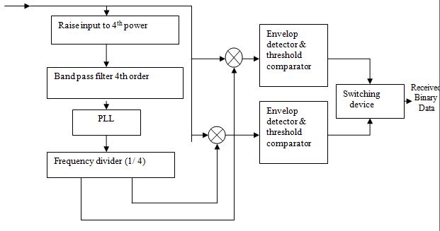
Figure 7.1: DETECTION
7.4 AWGN Channel
During transmission, the signal undergoes various degrading and distortion effects as it passes through the medium from transmitter to receiver. This medium is commonly referred to as the channel. Channel effects include but are not limited to noise, interference, linear and non linear distortion and attenuation. These effects are contributed by a wide verity of sources including solar radiation, weather and signal from adjacent channels. But many of the prominent effects originate from the components in the receiver. While many of the effects can be greatly reduced by good system design, careful choice of filter parameters and coordination of frequency parameter usage with other users, noise and attenuation generally can not be avoided and are the largest contributors to signal distortion.
The most commonly used channel model to deal with noise is the additive white Gaussian noise (AWGN) channel model. The name results because the noise is simply added to the signal while the term white is used because the frequency content is equal across the entire spectrum. In reality this type of noise does not exists and is confined to a finite spectrum, but it is sufficiently useful for systems whose bandwidth are small compared to the noise power spectrum. When modeling a system across an AWGN channel, the noise must first be filtered to the channel prior to addition.
Chapter 8
RESULTS
8.1 SIMULATION
The section describes the performance of QPSK Modulation for speech.The simulation was done using MATLAB 7 platform.
All codes for this chapter are contained in Appendix A. An adaptive filter is used in these routines. All of the repeatedly used values such as cosine and sine are retrieved from look up tables to reduce computation load.
8.2 TRANSMITTER
A speech signal is transmitted through the entire system. In each case speech signals are obtained from the internet. These are short segments of speech data of 6-7 seconds. From the speech signal 30874 samples are taken.
These samples are then quantized. Here 4 bit PCM is used (as 8 bit or higher PCM takes longer time during the simulation) to obtain a total of 123496 bits from 30874 samples.
The bits are divided into even bits and odd bits using flip flop. Here for simplicity and for the purpose of better understanding only 8 bits are shown on the figure instead of 123496 bits. Consider that the bit sequence is 11000110.
The even bits (1010) are modulated using a carrier signal (sine wave) and odd bits (1001) are modulated using the same carrier signal with 90 degree phase shift (cosine wave). The modulation process is explained explicitly in the previous sections. In the case of odd data cosine wave represents 1 while cosine wave with 180 degree phase shift represents 0. On the other hand in the case of even data sine wave represents 1 and sine wave with 180 degree phase shift represents 0. The odd data and even data are modulated separately in this way and then added using a linear adder to obtain QPSK modulated signal. This signal is passed through a band pass filter and transmitted through the channel.
8.3 Channel and receiver
In this system AWGN channel is considered. As the signal passes through the channel it is corrupted by AWGN noise. AWGN command in MATLAB is used to generate this noise. Here SNR is taken sufficiently large to avoid possibility of bit errors. Bit error rate and the performance of the system depend highly on the SNR which is discussed later in this chapter. To remove this AWGN interference sequence from the received signal the signal is passed through an adaptive filter. The adaptive filter uses LMS algorithm which is explained explicitly in the previous sections. Then the desired signal is obtained.
This desired signal is then passed through the demodulation process. At first it is passed through a PLL to obtain necessary carrier signal. Here for simplicity the angle generated by PLL is considered zero. At one side this desired signal is demodulated with sine wave to obtain even data while on the other side it is demodulated by cosine wave to obtain odd data.
Then these signals are passed through corresponding envelop detector and threshold comparator to obtain odd data and even data. When data is greater than .75 then it detected as 1 on the other hand when data is less than .75 then it is detected as 0. After that a switching device is used to combine odd data and even data.
Then this bit stream is passed through the decoder and the received speech signal is obtained. This received signal can be heard using soundsc command
Here theoretical Eb/N0 vs. BER curve for QPSK is shown
CHAPTER-9
CONCLUSION
In this project the details of a digital communication system implementation using QPSK modulation and adaptive equalization have been discussed. Pulse-code modulation (PCM) is a digital representation of an analog signal where the magnitude of the signal is sampled regularly at uniform intervals, then quantized to a series of symbols in a numeric (usually binary) code. PCM can facilitate accurate reception even with severe noise or interference. An adaptive equalizer is an equalization filter that automatically adapts to time-varying properties of the communication channel. It is frequently used with coherent modulations. It is useful for estimating and suppressing AWGN interference. Lastly, QPSK is an efficient modulation scheme currently used by modem satellite communication links.
We studied QPSK modulation technique through out the project. Instead of using other modulation techniques such MSK, 8-QPSK, 16-QPSK etc we used 4-QPSK in this project. QPSK is a quaternary modulation method, while MSK is a binary modulation method. In QPSK, the I and Q components may change simultaneously, allowing transitions through the origin. In a hypothetical system with infinite bandwidth, these transitions occur instantaneously; however, in a practical band-limited system (in particular, a system using a Nyquist filter) these transitions take a finite amount of time. This results in a signal with a non-constant envelope. MSK performed in such a way that the transitions occur around the unit circle in the complex plane, resulting in a true constant-envelope signal. Using 8-QPSK and 16-QPSK techniques higher data rate and higher spectral efficiency can be achieved but BER also increases. The performance of MSK, 8-QPSK, 16-QPSK techniques is better but implementation of these techniques is complex. 4-QPSK is simpler and easy to implement. Its spectral efficiency is not higher than that of 8-QPSK, 16-QPSK but it provides lower BER. In this project we performed the simulation of 4-QPSK modulation technique using MATLAB platform accurately and without any error. The system is flexible enough in accommodating any speech signal or analog signal. Digital communication systems can be implemented using QPSK modulation.